12. Finding signal and defining background | Background rate computation Analysis
With the CAST data fully reconstructed and energy calibrated, it is time to define the methods used to extract axion candidates and derive a background rate from the data. We first introduce the likelihood cut method in sec. 12.1 to motivate the need for reference X-ray data from an X-ray tube. Such data, taken at the CAST Detector Lab (CDL) will be discussed in depth in sec. 12.2. We then see how the reference data is used in the likelihood method to act as an event classifier in sec. 12.3. As an alternative to the likelihood cut, we will introduce another classifier in the form of a simple artificial neural network in sec. 12.4. This is another in depth discussion, as the selection of the training data and verification is non-trivial. With both classifiers discussed, it is time to include all other Septemboard detector features as additional vetoes in sec. 12.5. At the very end we will look at background rates for different cases, sec. 12.6, motivating the approach of our limit calculation in the next chapter.
Note: The methods discussed in this chapter are generally classifiers that predict how 'signal-like' a cluster is. Based on this prediction we will usually define a cut value as to keep a cluster as a potential signal. This means that if we apply the method to background data (that is, CAST data taken outside of solar trackings) we recover the 'background rate'; the irreducible amount of background left (at a certain efficiency), which is signal-like. If instead we apply the same methods to CAST solar tracking data we get instead a set of 'axion induced X-ray candidates'. 1 In the context of the chapter we commonly talk about "background rates", but the equivalent meaning in terms of tracking data and candidates should be kept in mind.
12.1. Likelihood method
The detection principle of the GridPix detector implies physically different kinds of events will have different geometrical shapes. An example can be seen in fig. 1(a), comparing the cluster eccentricity of \cefe calibration events with background data. This motivates usage of a geometry based approach to determine likely signal-like or background-like clusters. The method to distinguish the two types of events is a likelihood cut, based on the one in (Christoph Krieger 2018). It effectively assigns a single value to each cluster for the likelihood that it is a signal-like event.
Specifically, this likelihood method is based on three different geometric properties (also see sec. 9.4.2):
- the eccentricity \(ε\) of the cluster, determined by computing the long and short axis of the two dimensional cluster and then computing the ratio of the RMS of the projected positions of all active pixels within the cluster along each axis.
- the fraction of all pixels within a circle of the radius of one transverse RMS from the cluster center, \(f\).
- the length of the cluster (full extension along the long axis) divided by the transverse RMS, \(l\).
These variables are obviously highly correlated, but still provide a very good separation between the typical shapes of X-rays and background events. They mainly characterize the "spherical-ness" as well as the density near the center of the cluster, which is precisely the intuitive sense in which these type of events differ. For each of these properties we define a probability density function \(\mathcal{P}_i\), which can then be used to define the likelihood of a cluster with properties \((ε, f, l)\) to be signal-like:
\begin{equation} \label{eq:background:likelihood_def} \mathcal{L}(ε, f, l) = \mathcal{P}_{ε}(ε) \cdot \mathcal{P}_{f}(f) \cdot \mathcal{P}_l(l) \end{equation}where the subscript is denoting the individual probability density and the argument corresponds to the individual value of each property.
This raises the important question of what defines each individual probability density \(\mathcal{P}_i\). In principle it can be defined by computing a normalized density distribution of a known dataset, which contains representative signal-like data. The \cefe calibration data from CAST contains such representative data, if not for one problem: the properties used in the likelihood method are energy dependent, as seen in fig. 1(b), a comparison of the eccentricity of X-rays from the photopeak of the \cefe calibration source compared to those from the escape peak. The CAST calibration data can only characterize two different energies, but the expected axion signal is a (model dependent) continuous spectrum.
For this reason data was taken using an X-ray tube with 8 different target / filter combinations to provide the needed data to compute likelihood distributions for X-rays of a range of different energies. The details will be discussed in the next section, 12.2.


12.1.1. Generate plot of eccentricity signal vs. background extended
We will now generate a plot comparing the eccentricity of signal events from calibration data to background events. In addition another comparison will be made between photopeak photons and escape peak photons to show that events at different energies have different shapes, motivating the need for the X-ray tube data at different energies.
    import ggplotnim, nimhdf5
import ingrid / [tos_helpers, ingrid_types]

proc read  (f: string, run: int  ): DataFrame =
  withH5(f, "r"  ):
    result = h5f.readRunDsets(
      run = run,
      chipDsets = some(  (chip: 3, dsets: @[  "eccentricity", "centerX", "centerY", "energyFromCharge"  ]  )  )
    )

proc main  (calib, back: string  ) =

  #   read data from each file, one fixed run with good statistics
  #   cut on silver region
  let dfC = read(calib, 128  )
  let dfB = read(back, 124  )
  var df = bind_rows(  [  (  "Calibration", dfC), (  "Background", dfB)  ], "Type"  )
    .filter(f{  float -> bool: inRegion(`centerX`, `centerY`, crSilver)  },
            f{  float: `eccentricity` < 10.0  }  )
  ggplot(df, aes(  "eccentricity", fill = "Type"  )  ) +
    #  geom_histogram(bins = 100,
    #                 hdKind = hdOutline,
    #                 position = "identity",
    #                 alpha = 0.5,
    #                 density = true) +
    xlab(  "Eccentricity"  ) + ylab(  "Density"  ) +
    geom_density(color = "black", size = 1.0, alpha = 0.7, normalize = true  ) +
    ggtitle(  "Eccentricity of calibration and background data"  ) +
    themeLatex(fWidth = 0.5, width = 600, baseTheme = sideBySide) +
    margin(left = 2.2, right = 5.2  ) +
    ggsave(  "Figs/background/eccentricity_calibration_background.pdf", useTeX = true, standalone = true  )

  proc splitPeaks  (x: float  ): string =
    if x >= 2.75 and x <= 3.25:
      "Escapepeak"
    elif x >= 5.55 and x <= 6.25:
      "Photopeak"
    else:
      "Unclear"

  let dfP = dfC
      .mutate(f{  float: "Peak" ~ splitPeaks(`energyFromCharge`)  }  )
      .filter(f{  string: `Peak` != "Unclear"  },
              f{`eccentricity` <= 2.0  }  )
  ggplot(dfP, aes(  "eccentricity", fill = "Peak"  )  ) +
    #  geom_histogram(bins = 50,
    #                 hdKind = hdOutline,
    #                 position = "identity",
    #                 alpha = 0.5,
    #                 density = true) +
    xlab(  "Eccentricity"  ) + ylab(  "Density"  ) +
    geom_density(color = "black", size = 1.0, alpha = 0.7, normalize = true  ) +
    ggtitle(r"$^{55}\text{Fe}$ photopeak (5.9 keV) and escapepeak (3 keV)"  ) +
    themeLatex(fWidth = 0.5, width = 600, baseTheme = sideBySide) +
    margin(left = 2.2, right = 5.2  ) +
    ggsave(  "Figs/background/eccentricity_photo_escape_peak.pdf", useTeX = true, standalone = true  )

when isMainModule:
  import cligen
  dispatch main
yielding
and
12.2. CAST Detector Lab
In this section we will cover the X-ray tube data taken at the CAST Detector Lab (CDL) at CERN. First, we will show the setup in sec. 12.2.1. Next the different target / filter combinations that were used will be discussed and the measurements presented in sec. 12.2.2. These measurements then are used to define the probability densities for the likelihood method, see sec. 12.2.5. Further, in sec. 12.2.6, we cover a few more details on a linear interpolation we perform to compute a likelihood distribution at an arbitrary energy. And finally, they can be used to measure the energy resolution of the detector at different energies, sec. 12.2.9.
The data presented here was also part of the master thesis of Hendrik Schmick (Schmick 2019). Further, the selection of lines and approach follows the ideas used for the single GridPix detector in (Christoph Krieger 2018) with some notable differences. For a reasoning for one particular difference in terms of data treatment, see appendix 27.
Note: in the course of the CDL related sections the term target/filter combination (implicitly including the used high voltage setting) is used interchangeably with the main fluorescence line (or just 'the fluorescence line') targeted in a specific measurement. Be careful while reading about applied high voltages in \(\si{kV}\) and energies in \(\si{keV}\). The produced fluorescence lines typically have about 'half' the energy in \(\si{keV}\) as the applied voltage in \(\si{kV}\). See tab. 19 in sec. 12.2.2 for the precise relation.
12.2.1. CDL setup
The CAST detector lab provides a vacuum test stand, which contains an X-ray tube. A Micromegas-like detector can easily be mounted to the rear end of the test stand. An X-ray tube uses a filament to produce free electrons, which are then accelerated with a high voltage of the order of multiple \(\si{kV}\). The main part of the setup is a rotateable wheel inside the vacuum chamber, which contains a set of 18 different positions with 8 different target materials, as seen in tab. 17. The highly energetic electrons interacting with the target material generate a continuous Bremsstrahlung spectrum with characteristic lines depending on the target. A second rotateable wheel contains a set of 11 different filters, see tab. 18. These can be used to filter out undesired parts of the generated spectrum by choosing a filter that is opaque in the those energy ranges.
As mentioned previously in sec. 10.1, the detector was dismounted from CAST in Feb. 2019 and installed in the CAST detector lab on . The week from to X-ray tube data was taken in the CDL.
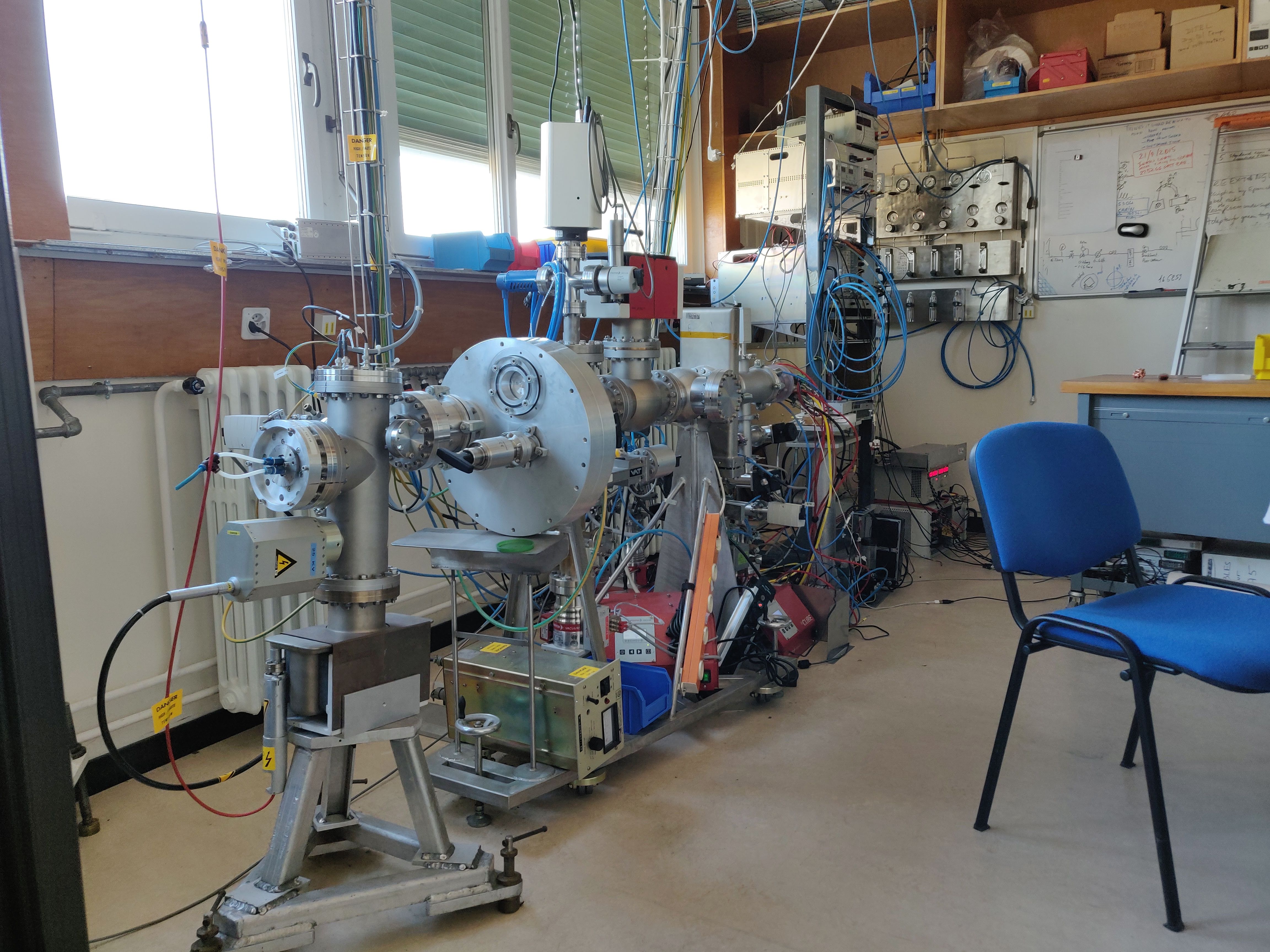
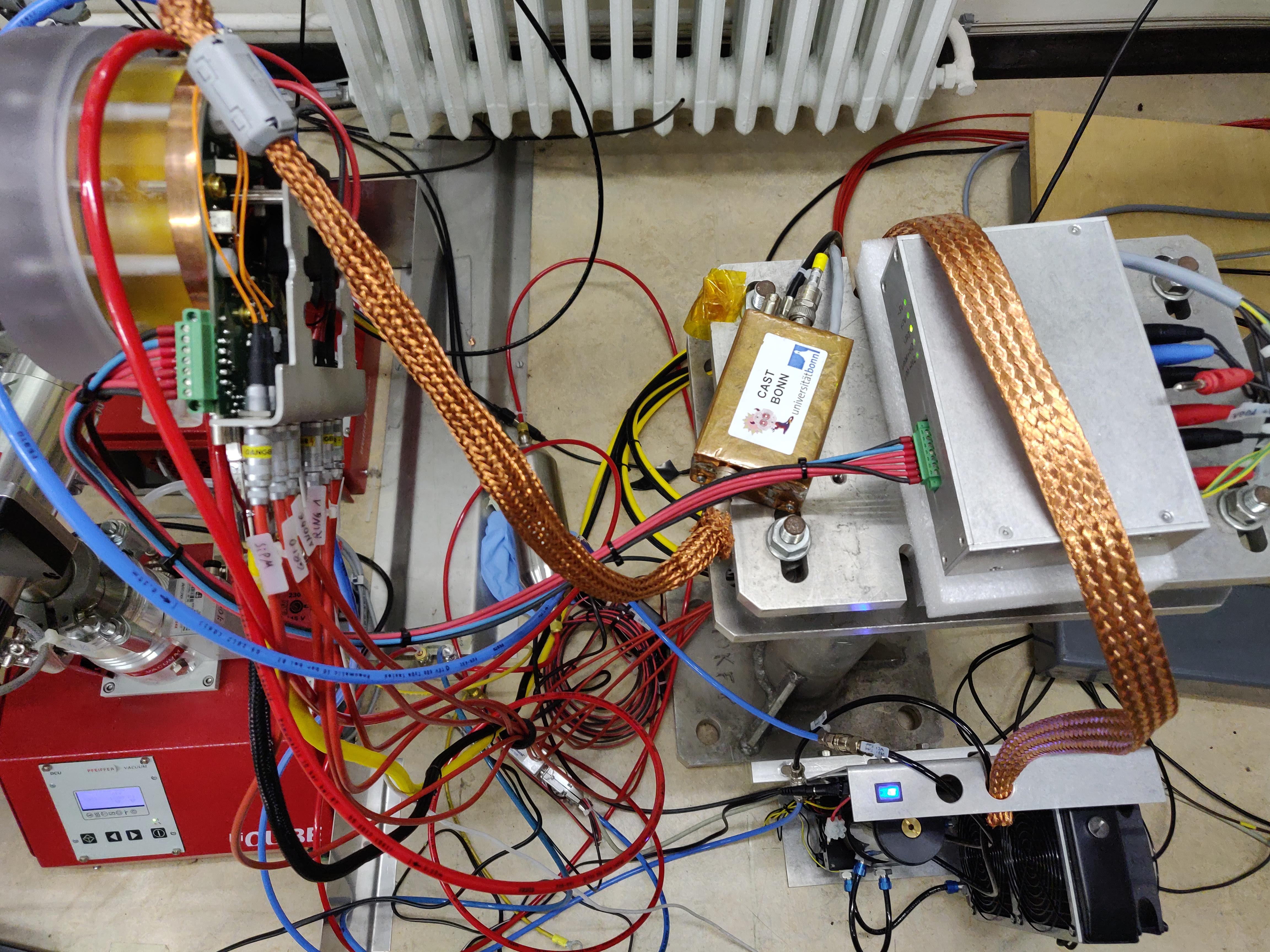
Fig. 2(a) shows the whole vacuum test stand, which contains the X-ray tube on the front left end and the Septemboard detector installed on the rear right, visible by the red HV cables and yellow HDMI cable. In fig. 2(b) we see the whole detector part from above, with the Septemboard detector installed to the vacuum test stand on the left side. The water cooling system is seen in the bottom right, with the power supply above that. The copper shielded box slightly right of the center is the Ortec pre-amplifier of the FADC, which is connected via a heavily shielded LEMO cable to the Septemboard detector. This cable was available in the CAST detector lab and proved invaluable for the measurements as it essentially removed any noise visible in the FADC signals (compared to the significant noise issues encountered at CAST, sec. 10.5.1). Given the activation threshold of the FADC with CAST amplifier settings (see sec. 11.4.2) at around \(\SI{2}{keV}\), the amplification needed to be adjusted in the CDL on a per-target basis. The shielded cable allowed the FADC to even act as a trigger for \(\SI{277}{eV}\) \(\ce{C}_{Kα}\) X-rays without any noise problems. 2
| Target Material | Position |
|---|---|
| Ti | 1 |
| Ag | 2 |
| Mn | 3 |
| C | 4 |
| BN | 5 |
| Au | 6 |
| Al | 7 - 11 |
| Cu | 12 - 18 |
| Filter material | Position |
|---|---|
| Ni 0.1 mm | 1 |
| Al 5 µm | 2 |
| PP G12 (EPIC) | 3 |
| PP G12 (EPIC) | 4 |
| Cu 10 µm | 5 |
| Ag 5 µm (99.97%) AG000130/24 | 6 |
| Fe 50 µm | 7 |
| Mn foil 50 µm (98.7% + permanent polyester) | 8 |
| Co 50 µm (99.99%) CO0000200 | 9 |
| Cr 40 µm (99.99% + permanent polyester) | 10 |
| Ti 50 µm (99.97%) TI000315 | 11 |
12.2.2. CDL measurements
The measurements were performed with 8 different target and filter combinations, with a higher density towards lower energies due to the nature of the expected solar axion flux. For each target and filter at least two runs were measured, one with and one without using the FADC as a trigger. The latter was taken to collect more statistics in a shorter amount of time, as the FADC readout slows down the data taking speed due to increased dead time. Table 19 provides an overview of all data taking runs, the target, filter and HV setting, the main X-ray fluorescence line targeted and its energy. Finally, the mean position of the main fluorescence line in the charge spectrum and its width as determined by a fit is shown. As can be seen the position moves in some cases significantly between different runs, for example in case of the \(\ce{Cu}-\ce{Ni}\) measurements. Also within a single run some stronger variation can be seen, evident by the much larger line width for example in run \(\num{320}\) compared to \(\num{319}\). See appendix sec. 26.4 for all measured spectra (pixel and charge spectra), where each plot contains all runs for a target / filter combination. For example fig. #fig:appendix:cdl_charge_Cu-Ni-15kV_by_run shows runs 319, 320 and 345 of the \(\ce{Cu}-\ce{Ni}\) measurements at \(\SI{15}{kV}\) with the strong variation in charge position of the peak visible between the runs.
The variability both between runs for the same target and filter as well as within a run shows the detector was undergoing gas gain changes similar to the variations at CAST (sec. 11.2). With an understanding that the variation is correlated to the temperature this can be explained. The small laboratory underwent significant temperature changes due to the presence of 3 people, all running machines and freely opening and closing windows, in particular due to very warm temperatures relative to a typical February in Geneva. 3 Fig. 3 shows the calculated gas gains (based on \(\SI{90}{min}\) intervals) for each run colored by the target/filter combination. It undergoes a strong, almost exponential change over the course of the data taking campaign. Because of this variation between runs, each run is treated fully separately in contrast to (Christoph Krieger 2018), where all runs for one target / filter combination were combined.

Fortunately, this significant change of gas gain does not have an impact on the distributions of the cluster properties. See appendix 27.1 for comparisons of the cluster properties of the different runs (and thus different gas gains) for each target and filter combination.
As the main purpose is to use the CDL data to generate reference distributions for certain cluster properties, the relevant clusters that correspond to known X-ray energies must be extracted from the data. This is done in two different ways:
- A set of fixed cuts (one set for each target/filter combination) is applied to each run, as presented in tab. 20. This is the same set as used in (Christoph Krieger 2018). Its main purpose is to remove events with multiple clusters and potential background contributions.
- By cutting around the main fluorescence line in the charge spectrum in a \(3σ\) region, for which the spectrum needs to be fitted with the expected lines, see sec. 12.2.3. This is done on a run-by-run basis.
The remaining data after both sets of cuts can then be combined for each target/filter combination to make up the distributions for the cluster properties as needed for the likelihood method.
For a reference of the X-ray fluorescence lines (for more exact values and \(\alpha_1\), \(\alpha_2\) values etc.) see tab. 1. The used EPIC filter refers to a filter developed for the EPIC camera of the XMM-Newton telescope. It is a bilayer of \(\SI{1600}{\angstrom}\) polyimide and \(\SI{800}{\angstrom}\) aluminium. For more information about the EPIC filters see references (Strüder et al. 2001; Turner, M. J. L. et al. 2001; Barbera et al. 2003, 2016), in particular (Barbera et al. 2016) for an overview of the materials and production.
| Run | FADC? | Target | Filter | HV [kV] | Line | Energy [keV] | μ [e⁻] | σ [e⁻] | σ/μ |
|---|---|---|---|---|---|---|---|---|---|
| 319 | y | Cu | Ni | 15 | \(\ce{Cu}\) \(\text{K}_{\alpha}\) | 8.04 | \(\num{9.509(21)e+05}\) | \(\num{7.82(18)e+04}\) | \(\num{8.22(19)e-02}\) |
| 320 | n | Cu | Ni | 15 | \(\num{9.102(22)e+05}\) | \(\num{1.010(19)e+05}\) | \(\num{1.110(21)e-01}\) | ||
| 345 | y | Cu | Ni | 15 | \(\num{6.680(12)e+05}\) | \(\num{7.15(11)e+04}\) | \(\num{1.070(16)e-01}\) | ||
| 315 | y | Mn | Cr | 12 | \(\ce{Mn}\) \(\text{K}_{\alpha}\) | 5.89 | \(\num{6.321(29)e+05}\) | \(\num{9.44(26)e+04}\) | \(\num{1.494(41)e-01}\) |
| 323 | n | Mn | Cr | 12 | \(\num{6.328(11)e+05}\) | \(\num{7.225(89)e+04}\) | \(\num{1.142(14)e-01}\) | ||
| 347 | y | Mn | Cr | 12 | \(\num{4.956(10)e+05}\) | \(\num{6.211(82)e+04}\) | \(\num{1.253(17)e-01}\) | ||
| 325 | y | Ti | Ti | 9 | \(\ce{Ti}\) \(\text{K}_{\alpha}\) | 4.51 | \(\num{4.83(31)e+05}\) | \(\num{4.87(83)e+04}\) | \(\num{1.01(18)e-01}\) |
| 326 | n | Ti | Ti | 9 | \(\num{4.615(87)e+05}\) | \(\num{4.93(25)e+04}\) | \(\num{1.068(57)e-01}\) | ||
| 349 | y | Ti | Ti | 9 | \(\num{3.90(23)e+05}\) | \(\num{4.57(57)e+04}\) | \(\num{1.17(16)e-01}\) | ||
| 328 | y | Ag | Ag | 6 | \(\ce{Ag}\) \(\text{L}_{\alpha}\) | 2.98 | \(\num{3.0682(97)e+05}\) | \(\num{3.935(79)e+04}\) | \(\num{1.283(26)e-01}\) |
| 329 | n | Ag | Ag | 6 | \(\num{3.0349(51)e+05}\) | \(\num{4.004(40)e+04}\) | \(\num{1.319(13)e-01}\) | ||
| 351 | y | Ag | Ag | 6 | \(\num{2.5432(63)e+05}\) | \(\num{3.545(49)e+04}\) | \(\num{1.394(20)e-01}\) | ||
| 332 | y | Al | Al | 4 | \(\ce{Al}\) \(\text{K}_{\alpha}\) | 1.49 | \(\num{1.4868(50)e+05}\) | \(\num{2.027(38)e+04}\) | \(\num{1.364(26)e-01}\) |
| 333 | n | Al | Al | 4 | \(\num{1.3544(30)e+05}\) | \(\num{2.539(24)e+04}\) | \(\num{1.875(18)e-01}\) | ||
| 335 | y | Cu | EPIC | 2 | \(\ce{Cu}\) \(\text{L}_{\alpha}\) | 0.930 | \(\num{8.885(99)e+04}\) | \(\num{1.71(11)e+04}\) | \(\num{1.93(13)e-01}\) |
| 336 | n | Cu | EPIC | 2 | \(\num{7.777(94)e+04}\) | \(\num{2.39(14)e+04}\) | \(\num{3.08(19)e-01}\) | ||
| 337 | n | Cu | EPIC | 2 | \(\num{7.86(15)e+04}\) | \(\num{2.47(11)e+04}\) | \(\num{3.14(15)e-01}\) | ||
| 339 | y | Cu | EPIC | 0.9 | \(\ce{O }\) \(\text{K}_{\alpha}\) | 0.525 | \(\num{5.77(11)e+04}\) | \(\num{1.38(22)e+04}\) | \(\num{2.39(39)e-01}\) |
| 340 | n | Cu | EPIC | 0.9 | \(\num{4.778(31)e+04}\) | \(\num{1.230(50)e+04}\) | \(\num{2.58(11)e-01}\) | ||
| 342 | y | C | EPIC | 0.6 | \(\ce{C }\) \(\text{K}_{\alpha}\) | 0.277 | \(\num{4.346(36)e+04}\) | \(\num{1.223(29)e+04}\) | \(\num{2.814(70)e-01}\) |
| 343 | n | C | EPIC | 0.6 | \(\num{3.952(20)e+04}\) | \(\num{1.335(14)e+04}\) | \(\num{3.379(40)e-01}\) |
| Target | Filter | line | HV | length | RMSTmin | RMSTmax | eccentricity |
|---|---|---|---|---|---|---|---|
| Cu | Ni | \(\ce{Cu}\) \(\text{K}_{\alpha}\) | 15 | 0.1 | 1.0 | 1.3 | |
| Mn | Cr | \(\ce{Mn}\) \(\text{K}_{\alpha}\) | 12 | 0.1 | 1.0 | 1.3 | |
| Ti | Ti | \(\ce{Ti}\) \(\text{K}_{\alpha}\) | 9 | 0.1 | 1.0 | 1.3 | |
| Ag | Ag | \(\ce{Ag}\) \(\text{L}_{\alpha}\) | 6 | 6.0 | 0.1 | 1.0 | 1.4 |
| Al | Al | \(\ce{Al}\) \(\text{K}_{\alpha}\) | 4 | 0.1 | 1.1 | 2.0 | |
| Cu | EPIC | \(\ce{Cu}\) \(\text{L}_{\alpha}\) | 2 | 0.1 | 1.1 | 2.0 | |
| Cu | EPIC | \(\ce{O }\) \(\text{K}_{\alpha}\) | 0.9 | 0.1 | 1.1 | 2.0 | |
| C | EPIC | \(\ce{C }\) \(\text{K}_{\alpha}\) | 0.6 | 6.0 | 0.1 | 1.1 |
12.2.2.1. Table of fit lines extended
This is the full table.
| cuNi15 | mnCr12 | tiTi9 | agAg6 | alAl4 | cuEpic2 | cuEpic09 | cEpic06 |
|---|---|---|---|---|---|---|---|
| \(\text{EG}(\ce{Cu}_{Kα})\) | \(\text{EG}(\ce{Mn}_{Kα})\) | \(\text{EG}(\ce{Ti}_{Kα})\) | \(\text{EG}(\ce{Ag}_{Lα})\) | \(\text{EG}(Al_{Kα})\) | \(\text{G}(\ce{Cu}_{Lα})\) | \(\text{G}(O_{Kα})\) | \(\text{G}(\ce{C}_{Kα})\) |
| \(\text{EG}(\ce{Cu}^{\text{esc}})\) | \(\text{G}(\ce{Mn}^{\text{esc}})\) | \(\text{G}(\ce{Ti}^{\text{esc}}_{Kα})\) | G: | G: | #G: | G: | |
| #name = \(\ce{Ti}^{\text{esc}}_{Kα}\) | name = \(\ce{Ag}_{Lβ}\) | name = \(\ce{Cu}_{Lβ}\) | # name = \(\ce{C}_{Kα}\) | name = \(\ce{O}_{Kα}\) | |||
| # \(μ = eμ(\ce{Ti}_{Kα}) · \frac{1.537}{4.511}\) | \(N = eN(\ce{Ag}_{Lα}) · 0.1\) | \(N = N(\ce{Cu}_{Lα}) / 5.0\) | # \(μ = μ(O_{Kα}) · (0.277/0.525)\) | \(μ = μ(\ce{C}_{Kα}) · \frac{0.525}{0.277}\) | |||
| G: | \(μ = eμ(\ce{Ag}_{Lα}) · \frac{3.151}{2.984}\) | \(μ = μ(\ce{Cu}_{Lα}) · \frac{0.9498}{0.9297}\) | # \(σ = σ(O_{Kα})\) | \(σ = σ(\ce{C}_{Kα})\) | |||
| name = \(\ce{Ti}^{\text{esc}}_{Kβ}\) | \(σ = eσ(\ce{Ag}_{Lα})\) | \(σ = σ(\ce{Cu}_{Lα})\) | #G: | ||||
| \(μ = eμ(\ce{Ti}_{Kα}) · \frac{1.959}{4.511}\) | G: | # name = \(\ce{Fe}_{Lα}β\) | |||||
| \(σ = σ(\ce{Ti}^{\text{esc}}_{Kα})\) | name = \(\ce{O}_{Kα}\) | # \(μ = μ(O_{Kα}) · \frac{0.71}{0.525}\) | |||||
| G: | \(N = N(\ce{Cu}_{Lα}) / 3.5\) | # \(σ = σ(O_{Kα})\) | |||||
| name = \(\ce{Ti}_{Kβ}\) | \(μ = μ(\ce{Cu}_{Lα}) · \frac{0.5249}{0.9297}\) | #G: | |||||
| \(μ = eμ(\ce{Ti}_{Kα}) · \frac{4.932}{4.511}\) | \(σ = σ(\ce{Cu}_{Lα}) / 2.0\) | # name = \(\ce{Ni}_{Lα}β\) | |||||
| \(σ = eσ(\ce{Ti}_{Kα})\) | # \(μ = μ(O_{Kα}) · \frac{0.86}{0.525}\) | ||||||
| cuNi15 Q | mnCr12 Q | tiTi9 Q | agAg6 Q | alAl4 Q | cuEpic2 Q | cuEpic09 Q | cEpic06 Q |
| \(\text{G}(\ce{Cu}_{Kα})\) | \(\text{G}(\ce{Mn}_{Kα})\) | \(\text{G}(\ce{Ti}_{Kα})\) | \(\text{G}(\ce{Ag}_{Lα})\) | \(\text{G}(Al_{Kα})\) | \(\text{G}(\ce{Cu}_{Lα})\) | \(\text{G}(O_{Kα})\) | \(\text{G}(\ce{C}_{Kα})\) |
| \(\text{G}(\ce{Cu}^{\text{esc}})\) | \(\text{G}(\ce{Mn}^{\text{esc}})\) | \(\text{G}(\ce{Ti}^{\text{esc}}_{Kα})\) | G: | G: | G: | G: | |
| #name = \(\ce{Ti}^{\text{esc}}_{Kα}\) | name = \(\ce{Ag}_{Lβ}\) | name = \(\ce{Cu}_{Lβ}\) | name = \(\ce{C}_{Kα}\) | name = \(\ce{O}_{Kα}\) | |||
| # \(μ = eμ(\ce{Ti}_{Kα}) · \frac{1.537}{4.511}\) | \(N = N(\ce{Ag}_{Lα}) · 0.1\) | \(N = N(\ce{Cu}_{Lα}) / 5.0\) | \(N = N(O_{Kα}) / 10.0\) | \(μ = μ(\ce{C}_{Kα}) · \frac{0.525}{0.277}\) | |||
| G: | \(μ = μ(\ce{Ag}_{Lα}) · \frac{3.151}{2.984}\) | \(μ = μ(\ce{Cu}_{Lα}) · \frac{0.9498}{0.9297}\) | \(μ = μ(O_{Kα}) · \frac{277.0}{524.9}\) | \(σ = σ(\ce{C}_{Kα})\) | |||
| name = \(\ce{Ti}^{\text{esc}}_{Kβ}\) | \(σ = σ(\ce{Ag}_{Lα})\) | \(σ = σ(\ce{Cu}_{Lα})\) | \(σ = σ(O_{Kα})\) | ||||
| \(μ = μ(\ce{Ti}_{Kα}) · \frac{1.959}{4.511}\) | # $\text{G}: | ||||||
| \(σ = σ(\ce{Ti}^{\text{esc}}_{Kα})\) | # name = \(\ce{O}_{Kα}\) | ||||||
| G: | # \(N = N(\ce{Cu}_{Lα}) / 4.0\) | ||||||
| name = \(\ce{Ti}_{Kβ}\) | # \(μ = μ(\ce{Cu}_{Lα}) · \frac{0.5249}{0.9297}\) | ||||||
| \(μ = μ(\ce{Ti}_{Kα}) · \frac{4.932}{4.511}\) | # \(σ = σ(\ce{Cu}_{Lα}) / 2.0\) | ||||||
| \(σ = σ(\ce{Ti}_{Kα})\) |
12.2.2.2. Extra info on target materials extended
[X]EXTEND THIS TO INCLUDE CITATIONS[ ]ADD OUR OWN POLYIAMID + ALUMINUM TRANSMISSION PLOT -> 1600 Å polyimide + 800 Å Al -> Q: What do we use for the polyimide? Guess below text can tell us the atomic fractions in principle.
EPIC filters: https://www.cosmos.esa.int/web/xmm-newton/technical-details-epic section 6 about filters contains:
There are four filters in each EPIC camera. Two are thin filters made of 1600 Å of poly-imide film with 400 Å of aluminium evaporated on to one side; one is the medium filter made of the same material but with 800 Å of aluminium deposited on it; and one is the thick filter. This is made of 3300 Å thick Polypropylene with 1100 Å of aluminium and 450 Å of tin evaporated on the film.
i.e. the EPIC filters contain aluminum. That could explain why the Cu-EPIC 2kV data contains something that might be either aluminum fluorescence or at least just continuous spectrum that is not filtered due to the absorption edge of aluminum there!
Relevant references: (Strüder et al. 2001; Turner, M. J. L. et al. 2001; Barbera et al. 2003, 2016)
In particular (Barbera et al. 2016) contains much more details about the EPIC filters and its actual composition:
Filter manufacturing process The EPIC Thin and Medium filters manufactured by MOXTEX consist of a thin film of polyimide, with nominal thickness of 160 nm, coated with a single layer of aluminum whose nominal thickness is 40 nm for the Thin and 80 nm for the Medium filters, respectively. The polyimide thin films are produced by spin-coating of a polyamic acid (PAA) solution obtained by dissolving two precursor monomers (an anhydride and an amine) in an organic polar solvent. For the EPIC Thin and Medium filters the two precursors are the Biphenyldianhydride (BPDA) and the p-Phenyldiamine (PDA) (Dupont PI-2610), and the solvent is N-methyl-2-pyrrolidone (NMP) and Propylene Glycol Monomethyl Ether (Dupont T9040 thinner). To convert the PAA into polyimide, the solution is heated up to remove the NMP and to induce the imidization through the evaporation of water molecules. The film thickness is controlled by spin coating parameters, PAA viscosity, and curing temperature [19]. The polyimide thin membrane is attached with epoxy onto a transfer ring and the aluminum is evaporated in a few runs, distributed over 2–3 days, each one depositing a metal layer of about 20 nm thickness.
The EPIC Thin and Medium flight qualified filters have been manufactured during a period of 1 year, from January’96 to January’97. Table 1 lists the full set of flight-qualified filters (Flight Model and Flight Spare) delivered to the EPIC consortium, together with their most relevant parameters. Along with the production of the flight qualified filters, the prototypes and the qualification filters (not included in this list) have been manufactured and tested for the construction of the filter transmission model and to assess the stability in time of the Optical/UV transparency (opacity). Among these qualification filters are T4, G12, G18, and G19 that have been previously mentioned.
Further it states that 'G12' refers to the medium filter
UV/Vis transmission measurements in the range 190–1000 nm have been performed between May 1997 and July 2002 on one Thin (T4) and one medium (G12) EPIC on-ground qualification filters to monitor their time stability [16].
PP G12 is the name written in the CDL documentation! Mystery solved.
12.2.2.3. Reconstruct all CDL data extended
Reconstructing all CDL data is done by either using runAnalysisChain
on the directory (currently not tested) or by manually running
raw_data_manipulation and reconstruction as follows:
Take note that you may change the paths of course. The paths chosen here are those in use during the writing process of the thesis.
    cd ~/CastData/data/CDL_2019
raw_data_manipulation -p . -r Xray -o ~/CastData/data/CDL_2019/CDL_2019_Raw.h5
And now for the reconstruction:
    cd ~/CastData/data/CDL_2019
reconstruction -i ~/CastData/data/CDL_2019/CDL_2019_Raw.h5 -o ~/CastData/data/CDL_2019/CDL_2019_Reco.h5
reconstruction -i ~/CastData/data/CDL_2019/CDL_2019_Reco.h5 --only_charge
reconstruction -i ~/CastData/data/CDL_2019/CDL_2019_Reco.h5 --only_fadc
reconstruction -i ~/CastData/data/CDL_2019/CDL_2019_Reco.h5 --only_gas_gain
reconstruction -i ~/CastData/data/CDL_2019/CDL_2019_Reco.h5 --only_energy_from_e
At this point the reconstructed CDL H5 file is generally done and ready to be used in the next section.
12.2.2.4. Generate plots and tables for this section extended
To generate the plots of the above section (and much more) as well as
the table summarizing all the runs and their fits, we continue
with the cdl_spectrum_creation tool as follows:
Make sure the config file uses fitByRun to reproduce the same plots!
ESCAPE_LATEX performs replacement of characters like & used in
titles.
    F_WIDTH=0.9 ESCAPE_LATEX=true USE_TEX=true \
            cdl_spectrum_creation \
            -i ~/CastData/data/CDL_2019/CDL_2019_Reco.h5 \
            --cutcdl --dumpAccurate --hideNloptFit \
            --plotPath ~/phd/Figs/CDL/fWidth0.9/
Note:
This generates lots of plots, all placed in the output directory. The
fWidth0.9 subdirectory is because here we wish to produce them with
slightly smaller fonts as the single charge spectrum we use in the
next section is inserted standalone.
Among them are:
- plots of the target / filter kinds with all fits and the raw / cut data as histogram
- plots of histograms of the raw data split by run -> useful to see the detector variability!
- energy resolution plot
- peak position of hits / charge vs energy (to see if indeed linear)
- calibrated, normalized histogram / kde plot of the target/filter combinations in energy (calibrated using the main line that was fitted)
- ridgeline plots of KDEs of all the geometric cluster properties split by target/filter kind and run
- gas gain of each gas gain slice in the CDL data, split by run & target filter kind
- temperature data of those CDL runs that contain it
- finally it generates the (almost complete) tables as shown in the above section for the data overview including μ, σ and μ/σ
Note about temperature plots:
-

 -> This plot including the IMB temperature shows us precisely what
we expect: the temperature of the IMB and the Septemboard is
directly related and just an offset of one another. This is very
valuable information to have as a reference
-> This plot including the IMB temperature shows us precisely what
we expect: the temperature of the IMB and the Septemboard is
directly related and just an offset of one another. This is very
valuable information to have as a reference-

-

As we ran the command from /tmp/ the output plots will be in a
/tmp/out/CDL* directory. We copy over the generated files files
including calibrated_cdl_energy_histos.pdf and
calibrated_cdl_energy_kde.pdf here to /phd/Figs/CDL/.
Finally, running the code snippet as mentioned above also produces table 19 as well as the equivalent for the pixel spectra and writes them to stdout at the end!
12.2.2.5. Generate the calibration-cdl-2018.h5 file extended
This is also done using the cdl_spectrum_creation. Assuming the
reconstructed CDL H5 file exists, it is as simple as:
  cdl_spectrum_creation -i ~/CastData/data/CDL_2019/CDL_2019_Reco.h5 --genCdlFile \
                      --outfile ~/CastData/data/CDL_2019/calibration-cdl
which generates calibration-cdl-2018.h5 for us.
Make sure the config file uses fitByRun to reproduce the same plots!
12.2.2.6. Get the table of fit lines from code extended
Our code cdl_spectrum_creation can be used to output the final
fitting functions in a format like the table inserted in the main
text, thanks to using a CT declarative definition of the fit
functions.
We do this by running:
cdl_spectrum_creation --printFunctions
12.2.2.7. Historical weather data for Geneva during CDL data taking extended
More or less location of CDL (side of building 17 at Meyrin CERN site):
46.22965, 6.04984
(https://www.openstreetmap.org/search?whereami=1&query=46.22965%2C6.04984#map=19/46.22965/6.04984)
Here we can see historic weather data plots from Meyrin from the relevant time range: https://meteostat.net/en/place/ch/meyrin?s=06700&t=2019-02-15/2019-02-21
This at least proves the weather was indeed very nice outside, sunny and over 10°C peak temperatures during the day!
I exported the data and it's available here: ./resources/weather_data_meyrin_cdl_data_taking.csv
Legend of the columns:
| # | Column | Description |
|---|---|---|
| 1 | time | Time |
| 2 | temp | Temperature |
| 3 | dwpt | Dew Point |
| 4 | rhum | Relative Humidity |
| 5 | prcp | Total Precipitation |
| 6 | snow | Snow Depth |
| 7 | wdir | Wind Direction |
| 8 | wspd | Wind Speed |
| 9 | wpgt | Peak Gust |
| 10 | pres | Air Pressure |
| 11 | tsun | Sunshine Duration |
| 12 | coco | Weather Condition Code |
    import ggplotnim, times
var df = readCsv(  "/home/basti/phd/resources/weather_data_meyrin_cdl_data_taking.csv"  )
  .mutate(f{  string -> int: "timestamp" ~ parseTime(`time`, "yyyy-MM-dd HH:mm:ss", local()  ).toUnix()  }  )
  .rename(f{  "Temperature [°C]" <- "temp"  }, f{  "Pressure [mbar]" <- "pres"  }  )
df = df.gather(  [  "Temperature [°C]", "Pressure [mbar]"  ], "Data", "Value"  )
echo df
ggplot(df, aes(  "timestamp", "Value", color = "Data"  )  ) +
  facet_wrap(  "Data", scales = "free"  ) +
  facetMargin(  0.5  ) +
  geom_line() +
  xlab(  "Date", rotate = -45.0, alignTo = "right", margin = 2.0  ) +
  margin(bottom = 2.5, right = 4.75  ) +
  legendPosition(  0.84, 0.0  ) +
  scale_x_date(isTimestamp = true,
               dateSpacing = initDuration(hours = 12  ),
               formatString = "yyyy-MM-dd HH:mm",
               timeZone = local()  ) +
  ggtitle(  "Meyrin, Geneva weather during CDL data taking campaign"  ) +
  ggsave(  "/home/basti/phd/Figs/CDL/weather_meyrin_during_cdl_data_taking.pdf", width = 1000, height = 600  )
The weather during the data taking campaign is shown in fig. 4. It's good to see my memory served me right.

12.2.3. Charge spectra of the CDL data
To the spectra of each run of the charge data a mixture of Gaussian functions is fitted. 4
Specifically the Gaussian expressed as
\begin{equation} G(E; \mu, \sigma, N) = \frac{N}{\sqrt{2 \pi}} \exp\left(-\frac{(E - \mu)^2}{2\sigma^2}\right), \end{equation}is used and will be referenced as \(G\) with possible arguments from here on. Note that while the physical X-ray transition lines are Lorentzian shaped (Weisskopf and Wigner 1997), the lines as detected by a gaseous detector are entirely dominated by detector resolution, resulting in Gaussian lines. For other types of detectors used in X-ray fluorescence (XRF) analysis, convolutions of Lorentzian and Gaussian distributions are used (Huang and Lim 1986; Heckel and Scholz 1987), called pseudo Voigt functions (Roberts, Riddle, and Squier 1975; Gunnink 1977).
The functions fitted to the different spectra then depend on which fluorescence lines are visible. The full list of all combinations is shown in tab. 22. Typically each line that is expected from the choice of target, filter and chosen voltage is fitted, if it can be visually identified in the data. 5 If no 'argument' is shown in the table to \(G\) it means each parameter (\(N, μ, σ\)) is fitted. Any specific argument given implies that parameter is fixed relative to another parameter. For example \(μ^{\ce{Ag}}_{Lα}·\left(\frac{3.151}{2.984}\right)\) fixes the \(Lβ\) line of silver to the fit parameter \(μ^{\ce{Ag}}_{Lα}\) of the \(Lα\) line with a multiplicative shift based on the relative eneries of \(Lα\) to \(Lβ\). In some cases the amplitude is fixed between different lines where relative amplitudes cannot be easily predicted or determined, e.g. in one of the \(\ce{Cu}-\text{EPIC}\) runs, the \(\ce{C}_{Kα}\) line is fixed to a tenth of the \(\ce{O}_{Kα}\) line. This is done to get a good fit based on trial and error.
Finally, in both \(\ce{Cu}-\text{EPIC}\) lines two 'unknown' Gaussians are added to cover the behavior of the data at higher charges. The physical origin of this additional contribution is not entirely clear. The used EPIC filter contains an aluminum coating (Barbera et al. 2016). As such it has the aluminum absorption edge at about \(\SI{1.5}{keV}\), possibly matching the additional contribution for the \(\SI{2}{kV}\) dataset. Whether it is from a continuous part of the spectrum or a form of aluminum fluorescence is not clear however. This explanation does not work in the \(\SI{0.9}{kV}\) case, which is why the line is deemed 'unknown'. It may also be a contribution of the specific polyimide used in the EPIC filter (Barbera et al. 2016). Another possibility is it is a case of multi-cluster events, which are too close to be split, but with properties close enough to a single X-ray as to not be removed by the cleaning cuts (which gets more likely the lower the energy is).
The full set of all fits (including the pixel spectra) is shown in appendix 26.4. Fig. 5 shows the charge spectrum of the \(\ce{Ti}\) target and \(\ce{Ti}\) filter at \(\SI{9}{kV}\) for one of the runs. These plots show the raw data in the green histogram and the data left after application of the cleaning cuts (tab. 20) in the purple histogram. The black line is the result of the fit as described in tab. 22 with the resulting parameters shown in the box (parameters that were fixed are not shown). The black straight lines with grey error bands represent the \(3σ\) region around the main fluorescence line, which is used to extract those clusters likely from the fluorescence line and therefore known energy.

\footnotesize
| Target | Filter | HV [kV] | Fit functions |
|---|---|---|---|
| Cu | Ni | 15 | \(G^{\ce{Cu}}_{Kα} + G^{\ce{Cu}, \text{esc}}_{Kα}\) |
| Mn | Cr | 12 | \(G^{\ce{Mn}}_{Kα} + G^{\ce{Mn}, \text{esc}}_{Kα}\) |
| Ti | Ti | 9 | \(G^{\ce{Ti}}_{Kα} + G^{\ce{Ti}, \text{esc}}_{Kα} + G^{\ce{Ti}}_{Kβ}\left( μ^{\ce{Ti}}_{Kα}·\left(\frac{4.932}{4.511}\right), σ^{\ce{Ti}}_{Kα} \right) + G^{\ce{Ti}, \text{esc}}_{Kβ}\left( μ^{\ce{Ti}}_{Kα}·\left(\frac{1.959}{4.511}\right), σ^{\ce{Ti}, \text{esc}}_{Kα} \right)\) |
| Ag | Ag | 6 | \(G^{\ce{Ag}}_{Lα} + G^{\ce{Ag}}_{Lβ}\left( N^{\ce{Ag}}_{Lα}·0.56, μ^{\ce{Ag}}_{Lα}·\left(\frac{3.151}{2.984}\right), σ^{\ce{Ag}}_{Lα} \right)\) |
| Al | Al | 4 | \(G^{\ce{Al}}_{Kα}\) |
| Cu | EPIC | 2 | \(G^{\ce{Cu}}_{Lα} + G^{\ce{Cu}}_{Lβ}\left( N^{\ce{Cu}}_{Lα}·\left(\frac{0.65}{1.11}\right), μ^{\ce{Cu}}_{Lα}·\left(\frac{0.9498}{0.9297}\right), σ^{\ce{Cu}}_{Lα} \right) + G^{\ce{O}}_{Kα}\left( \frac{N^{\ce{Cu}}_{Lα}}{3.5}, μ^{\ce{Cu}}_{Lα}·\left(\frac{0.5249}{0.9297}\right), \frac{σ^{\ce{Cu}}_{Lα}}{2.0} \right) + G_{\text{unknown}}\) |
| Cu | EPIC | 0.9 | \(G^{\ce{O}}_{Kα} + G^{\ce{C}}_{Kα}\left( \frac{N^{\ce{O}}_{Kα}}{10.0}, μ^{\ce{O}}_{Kα}·\left(\frac{277.0}{524.9}\right), σ^{\ce{O}}_{Kα} \right) + G_{\text{unknown}}\) |
| C | EPIC | 0.6 | \(G^{\ce{C}}_{Kα} + G^{\ce{O}}_{Kα}\left( μ^{\ce{C}}_{Kα}·\left(\frac{0.525}{0.277}\right), σ^{\ce{C}}_{Kα} \right)\) |
\normalsize
12.2.3.1. Notes on implementation details of fit functions extended
[ ]REWRITE THE BELOW (much of that is irrelevant for the full thesis) -> Place into :noexport: section!
The exact implementation in use for both the gaussian:
The fitting was performed both with MPFit (Levenberg Marquardt C implementation) as a comparison, but mainly using NLopt (via https://github.com/Vindaar/nimnlopt). Specifically the gradient based "Method of Moving Asymptotes" algorithm was used (NLopt provides a large number of different minimization / maximization algorithms to choose from) to perform maximum likelihood estimation written in the form of a poisson distributed log likelihood \(\chi^2\):
where \(n_i\) is the number of events in bin \(i\) and \(y_i\) the model prediction of events in bin \(i\).
The required gradient was calculated simply using the symmetric derivative. Other algorithms and minimization functions were tried, but this proved to be the most reliable. See the implementation: https://github.com/Vindaar/TimepixAnalysis/blob/master/Analysis/ingrid/calibration.nim#L131-L162
12.2.3.2. Pixel spectra extended
In case of the pixel spectra the fit functions are generally very similar, but in some cases the regular Gaussian is replaced by an 'exponential Gaussian' defined as follows:
where the constant \(c\) is chosen such that the resulting function is continuous. The idea being that in the pixel spectra can have a longer exponential tail on the left side due to threshold effects and multiple electrons entering a single grid hole.
The implementation of the exponential Gaussian is found here: https://github.com/Vindaar/TimepixAnalysis/blob/master/Analysis/ingrid/calibration.nim#L182-L194
[ ]REPLACE LINKS SUCH AS THESE BY TAGGED VERSION AND NOT DIRECT INLINE LINKS
The full list of all fit combinations for the pixel spectra is shown in tab. 23. The fitting otherwise works the same way, using a non-linear least square fit both implemented by hand using MMA as well as a standard Levenberg-Marquardt fit.
| Target | Filter | HV [kV] | Fit functions |
|---|---|---|---|
| Cu | Ni | 15 | \(EG^{\ce{Cu}}_{Kα} + EG^{\ce{Cu}, \text{esc}}_{Kα}\) |
| Mn | Cr | 12 | \(EG^{\ce{Mn}}_{Kα} + G^{\ce{Mn}, \text{esc}}_{Kα}\) |
| Ti | Ti | 9 | \(EG^{\ce{Ti}}_{Kα} + G^{\ce{Ti}, \text{esc}}_{Kα} + G^{\ce{Ti}, \text{esc}}_{Kβ}\left( eμ^{\ce{Ti}}_{Kα}·(\frac{1.959}{4.511}), σ^{\ce{Ti}, \text{esc}}_{Kα} \right) + G^{\ce{Ti}}_{Kβ}\left( eμ^{\ce{Ti}}_{Kα}·(\frac{4.932}{4.511}), eσ^{\ce{Ti}}_{Kα} \right)\) |
| Ag | Ag | 6 | \(EG^{\ce{Ag}}_{Lα} + G^{\ce{Ag}}_{Lβ}\left( eN^{\ce{Ag}}_{Lα}·0.56, eμ^{\ce{Ag}}_{Lα}·(\frac{3.151}{2.984}), eσ^{\ce{Ag}}_{Lα} \right)\) |
| Al | Al | 4 | \(EG^{\ce{Al}}_{Kα}\) |
| Cu | EPIC | 2 | \(G^{\ce{Cu}}_{Lα} + G^{\ce{Cu}}_{Lβ}\left( N^{\ce{Cu}}_{Lα}·(\frac{0.65}{1.11}), μ^{\ce{Cu}}_{Lα}·(\frac{0.9498}{0.9297}), σ^{\ce{Cu}}_{Lα} \right) + G^{\ce{O}}_{Kα}\left( \frac{N^{\ce{Cu}}_{Lα}}{3.5}, μ^{\ce{Cu}}_{Lα}·(\frac{0.5249}{0.9297}), \frac{σ^{\ce{Cu}}_{Lα}}{2.0} \right) + G_{\text{unknown}}\) |
| Cu | EPIC | 0.9 | \(G^{\ce{O}}_{Kα} + G_{\text{unknown}}\) |
| C | EPIC | 0.6 | \(G^{\ce{C}}_{Kα} + G^{\ce{O}}_{Kα}\left( μ^{\ce{C}}_{Kα}·(\frac{0.525}{0.277}), σ^{\ce{C}}_{Kα} \right)\) |
12.2.3.3. Generate plot of charge spectrum extended
See sec. 12.2.2.4 for the commands used to generate all the plots for the pixel and charge spectra, including the one used in the above section.
12.2.4. Overview of CDL data in energy
With the fits to the charge spectra performed on a run-by-run basis, they can be utilized to calibrate the energy of each cluster in the data. 6 This is done by using the linear relationship between charge and energy and therefore using the charge of the main fluorescence line as computed from the fit. Each run is therefore self-calibrated (in contrast to our normal energy calibration approach 11.1). Fig. 6 shows normalized histograms of all CDL data after applying basic cuts and performing said energy calibrations.

12.2.5. Definition of the reference distributions
Having performed fits to all charge spectra of each run and the position of the main fluorescence line and its width determined, the reference distributions for the cluster properties entering the likelihood can be computed. By taking all clusters within the \(3σ\) bounds around the main fluorescence line of the data used for the fit, the dataset is selected. This guarantees to leave mainly X-rays of the targeted energy for each line in the dataset. As the fit is performed for each run separately, the \(3σ\) charge cut is performed run by run and then all data combined for each fluorescence line (target, filter & HV setting).
The desired reference distributions then are simply the normalized histograms of the clusters in each of the properties. With 8 targeted fluorescence lines and 3 properties this yields a total of 24 reference distributions. Each histogram is then interpreted as a probability density function (PDF) for clusters 'matching' (more on this in sec. 12.2.6) the energy of its fluorescence line. An overview of all the reference distributions is shown in fig. 7. We can see that all distributions tend to get wider towards lower energies (towards the top of the plot). This is expected and due to smaller clusters having less primary electrons and therefore statistical variations in geometric properties playing a more important role. 7 The binning shown in the figure is the exact binning used to define the PDF. In case of the fraction of pixels within a transverse RMS radius, bins with significantly higher counts are observed at low energies. This is not a binning artifact, but a result of the definition of the variable. The property computes the fraction of pixels that lie within a circle of the radius corresponding to the transverse RMS of the cluster around the cluster center (see fig. #fig:reco:property_explanations). At energies with few pixels in total, the integer nature of \(N\) or \(N+1\) primary electrons (active pixels) inside the radius becomes apparent.
The binning in the histograms is chosen by hand such that the binning is as fine as possible without leading to significant statistical fluctuations, as those would have a direct effect on the PDFs leading to unphysical effects on the probabilities. Ideally an approach of either an automatic bin selection algorithm or something like a kernel density estimation should be used. However, the latter is slightly problematic due to the integer effects in the low energies of the fraction in transverse RMS variable.
The summarized 'recipe' of the approach is therefore:
- apply cleaning cuts according to tab. 20,
- perform fits according to tab. 22,
- cut to the \(3σ\) region around the main fluorescence line of the performed fit (i.e. the first term in tab. 22),
- combine all remaining clusters for the same fluorescence line from each run,
- compute a histogram for each desired cluster property and each fluorescence line,
- normalize the histogram to define the reference distribution, \(\mathcal{P}_i\)

12.2.5.1. Generate ridgeline plot of all reference distributions extended
The ridgeline plot used in the above section is produced using
TimepixAnalysis/Plotting/plotCdl. See
sec. 12.2.6.1 for the exact commands as
more plots are produced used in other sections.
12.2.5.2. Generate plots for interpolated likelihood distribution and logL variable correlations [/] extended
In the main text I mentioned that the \(\ln\mathcal{L}\) variables are all very correlated. Let's create a few plots to look at how correlated they actually are. We'll generate scatter plots of the three variables against another, using a color scale for the third variable.
[ ]WRITE A FEW WORDS ABOUT THE PLOTS![X]Create a plot of the likelihood distributions interpolated over all energies! Well, it doesn't work in the way I thought, because obviously we cannot just compute the likelihood distributions directly! We can compute a likelihood value for a cluster at an arbitrary energy, but to get a likelihood distribution we'd need actual X-ray data at all energies! The closest we have to that is the general CDL data (not just the main peak & using correct energies for each cluster) -> Attempt to use the CDL data with only the cleaning cuts -> Question: Which tool do we add this to? Or separate here using CDL reconstructed data?
How much statistics do we even have if we end up splitting everything over 1000 energies? Like nothing… Done in:
 now where we compare the no morphing vs. the linear morphing
case. Much more interesting than I would have thought, because one
can clearly see the effect of the morphing on the logL values that
are computed!
This is a pretty nice result to showcase the morphing is actually
useful. Will be put into appendix and linked.
now where we compare the no morphing vs. the linear morphing
case. Much more interesting than I would have thought, because one
can clearly see the effect of the morphing on the logL values that
are computed!
This is a pretty nice result to showcase the morphing is actually
useful. Will be put into appendix and linked.
[X]ADD LINE SHOWING WHERE THE CUT VALUES ARE TO THE PLOT -> The hard corners in the interpolated data is because the reference distributions are already pre-binned of course! So if by just changing the bins slightly the ε cut value still lies in the same bin, of course we see a 'straight' line in energy. Hence a non smooth curve. We could replace this all:- either by a smooth KDE and interpolate based on that as an alternative. I should really try this, the only questionable issue is the fracRms distribution and its discrete features. However we don't actually guarantee in any way that in current approach the bins actually correspond to any fixed integer values. It is quite likely that the bins that show smaller/larger values are too wide/small!
- or by keeping everything as is, but then performing a spline interpolation on the distinct (logL, energy) pairs such that the result is a smooth logL value. "Better bang for buck" than doing full KDE and avoids the issue of discreteness in the fracRms distribution. Even though the interpolated values probably correspond to something as if the fracRms distribution had been smooth.
    import std / [os, strutils]
import ingrid / ingrid_types
import ingrid / private / [cdl_utils, cdl_cuts, hdf5_utils, likelihood_utils]
import pkg / [ggplotnim, nimhdf5]


const TpxDir = "/home/basti/CastData/ExternCode/TimepixAnalysis"
const cdl_runs_file = TpxDir / "resources/cdl_runs_2019.org"
const fname = "/home/basti/CastData/data/CDL_2019/CDL_2019_Reco.h5"
const cdlFile = "/home/basti/CastData/data/CDL_2019/calibration-cdl-2018.h5"
const dsets = @[  "totalCharge", "eccentricity", "lengthDivRmsTrans", "fractionInTransverseRms"  ]

proc calcEnergyFromFits  (df: DataFrame, fit_μ: float, tfKind: TargetFilterKind  ): DataFrame =
  ## Given the fit result of this data type & target/filter combination compute the energy
  ## of each cluster by using the mean position of the main peak and its known energy
  result = df
  result  [  "Target"  ] = $tfKind
  let invTab = getInverseXrayRefTable()
  let energies = getXrayFluorescenceLines()
  let lineEnergy = energies[invTab[$tfKind]  ]
  result = result.mutate(f{  float: "energy" ~ `totalCharge` / fit_μ * lineEnergy}  )

let h5f = H5open  (fname, "r"  )
var df = newDataFrame()
for tfKind in TargetFilterKind:
  for (run, grp) in tfRuns(h5f, tfKind, cdl_runs_file):
    var dfLoc = newDataFrame()
    for dset in dsets:
      if dfLoc.len == 0:
        dfLoc = toDf(  { dset : h5f.readCutCDL(run, 3, dset, tfKind, float64  ) }  )
      else:
        dfLoc[dset] = h5f.readCutCDL(run, 3, dset, tfKind, float64  )
    dfLoc[  "runNumber"  ] = run
    dfLoc[  "tfKind"  ] = $tfKind
    #   calculate energy from fit
    let fit_μ = grp.attrs[  "fit_μ", float  ]
    dfLoc = dfLoc.calcEnergyFromFits(fit_μ, tfKind)
    df.add dfLoc

proc calcInterp  (ctx: LikelihoodContext, df: DataFrame  ): DataFrame =
  #   walk all rows
  #   feed ecc, ldiv, frac into logL and return a DF with
  result = df.mutate(f{  float: "logL" ~ ctx.calcLikelihoodForEvent(`energy`,
                                                            `eccentricity`,
                                                            `lengthDivRmsTrans`,
                                                            `fractionInTransverseRms`)
  }  )

#   first make plots of 3 logL variables to see their correlations
ggplot(df, aes(  "eccentricity", "lengthDivRmsTrans", color = "fractionInTransverseRms"  )  ) +
  geom_point(size = 1.0  ) +
  ggtitle(  "lnL variables of all (cleaned) CDL data for correlations"  ) +
  ggsave(  "~/phd/Figs/background/correlation_ecc_ldiv_frac.pdf", dataAsBitmap = true  )

ggplot(df, aes(  "eccentricity", "fractionInTransverseRms", color = "lengthDivRmsTrans"  )  ) +
  geom_point(size = 1.0  ) +
  ggtitle(  "lnL variables of all (cleaned) CDL data for correlations"  ) +
  ggsave(  "~/phd/Figs/background/correlation_ecc_frac_ldiv.pdf", dataAsBitmap = true  )

ggplot(df, aes(  "lengthDivRmsTrans", "fractionInTransverseRms", color = "eccentricity"  )  ) +
  geom_point(size = 1.0  ) +
  ggtitle(  "lnL variables of all (cleaned) CDL data for correlations"  ) +
  ggsave(  "~/phd/Figs/background/correlation_ldiv_frac_ecc.pdf", dataAsBitmap = true  )


df = df.filter(f{`eccentricity` < 2.5  }  )
ggplot(df, aes(  "eccentricity", "lengthDivRmsTrans", color = "fractionInTransverseRms"  )  ) +
  geom_point(size = 1.0  ) +
  ggtitle(  "lnL variables of all (cleaned) CDL data for correlations (ε < 2.5)"  ) +
  ggsave(  "~/phd/Figs/background/correlation_ecc_ldiv_frac_ecc_smaller_2_5.pdf", dataAsBitmap = true  )

ggplot(df, aes(  "eccentricity", "fractionInTransverseRms", color = "lengthDivRmsTrans"  )  ) +
  geom_point(size = 1.0  ) +
  ggtitle(  "lnL variables of all (cleaned) CDL data for correlations (ε < 2.5)"  ) +
  ggsave(  "~/phd/Figs/background/correlation_ecc_frac_ldiv_ecc_smaller_2_5.pdf", dataAsBitmap = true  )

ggplot(df, aes(  "lengthDivRmsTrans", "fractionInTransverseRms", color = "eccentricity"  )  ) +
  geom_point(size = 1.0  ) +
  ggtitle(  "lnL variables of all (cleaned) CDL data for correlations (ε < 2.5)"  ) +
  ggsave(  "~/phd/Figs/background/correlation_ldiv_frac_ecc_ecc_smaller_2_5.pdf", dataAsBitmap = true  )


from std/sequtils import concat
#   now generate the plot of the logL values for all cleaned CDL data. We will compare the
#   case of no morphing with the linear morphing case
proc getLogL  (df: DataFrame, mk: MorphingKind  ): (  DataFrame, DataFrame  ) =
  let ctx = initLikelihoodContext(cdlFile, yr2018, crGold, igEnergyFromCharge, Timepix1, mk, useLnLCut = true  )
  var dfMorph = ctx.calcInterp(df)
  dfMorph[  "Morphing?"  ] = $mk
  let cutVals = ctx.calcCutValueTab()
  case cutVals.morphKind
  of mkNone:
    let lineEnergies = getEnergyBinning()
    let tab = getInverseXrayRefTable()
    var cuts = newSeq  [  float  ]()
    var energies = @[  0.0  ]
    var lastCut = Inf
    var lastE = Inf
    for k, v in tab:
      let cut = cutVals[k]
      if classify(lastCut) != fcInf:
        cuts.add lastCut
        energies.add lastE
      cuts.add cut
      lastCut = cut
      let E = lineEnergies[v]
      energies.add E
      lastE = E
    cuts.add cuts[^1  ] #   add last value again to draw line up
    echo energies.len, " vs ", cuts.len
    let dfCuts = toDf(  {energies, cuts, "Morphing?" : $cutVals.morphKind}  )
    result = (dfCuts, dfMorph)
  of mkLinear:
    let energies = concat(@[  0.0  ], cutVals.lnLCutEnergies, @[  20.0  ]  )
    let cutsSeq = cutVals.lnLCutValues.toSeq1D
    let cuts = concat(@[cutVals.lnLCutValues[  0  ]  ], cutsSeq, @[cutsSeq[^1  ]  ]  )
    let dfCuts = toDf(  {  "energies" : energies, "cuts" : cuts, "Morphing?" : $cutVals.morphKind}  )
    result = (dfCuts, dfMorph)

var dfMorph = newDataFrame()
let (dfCutsNone, dfNone) = getLogL(df, mkNone)
let (dfCutsLinear, dfLinear) = getLogL(df, mkLinear)
dfMorph.add dfNone
dfMorph.add dfLinear

var dfCuts = newDataFrame()
dfCuts.add dfCutsNone
dfCuts.add dfCutsLinear

#  dfCuts.showBrowser()

echo dfMorph
ggplot(dfMorph, aes(  "logL", "energy", color = factor(  "Target"  )  )  ) +
  facet_wrap(  "Morphing?"  ) +
  geom_point(size = 1.0  ) +
  geom_line(data = dfCuts, aes = aes(  "cuts", "energies"  )  ) + #   , color = "Morphing?")) +
  ggtitle(r"$\ln\mathcal{L}$ values of all (cleaned) CDL data against energy"  ) +
  themeLatex(fWidth = 0.9, width = 600, baseTheme = singlePlot) +
  ylab(  "Energy [keV]"  ) + xlab(r"$\ln\mathcal{L}$"  ) +
  ggsave(  "~/phd/Figs/background/logL_of_CDL_vs_energy.pdf", width = 1000, height = 600, dataAsBitmap = true  )
12.2.6. Definition of the likelihood distribution
With our reference distributions defined it is time to look back at the equation for the definition of the likelihood, eq. \eqref{eq:background:likelihood_def}.
Note: To avoid numerical issues dealing with very small probabilities, the actual relation evaluated numerically is the negative log of the likelihood:
\[ -\ln \mathcal{L}(ε, f, l) = - \ln \mathcal{P}_ε(ε) - \ln \mathcal{P}_f(f) - \ln \mathcal{P}_l(l). \]
By considering a single fluorescence line, the three reference distributions \(\mathcal{P}_i(i)\) make up the likelihood \(\mathcal{L}(ε, l, f)\) function for that energy; a function of the variables \(ε, f, l\). In order to use the likelihood function as a classifier for X-ray like clusters we need a one dimensional expression. This is where the likelihood distribution \(\mathfrak{L}\) comes in. We reuse all the clusters used to define the reference distributions \(\mathcal{P}_{ε,f,l}\) and compute their likelihood values \(\{ \mathcal{L}_j \}\), where \(j\) is the index of the \(j\text{-th}\) cluster. By then computing the histogram of the set of all these likelihood values, we obtain the likelihood distribution
\[ \mathfrak{L} = \text{histogram}\left( \{ \mathcal{L}_j \} \right). \]
All these distributions are shown in fig. 8 as negative log likelihood distributions. 8 We see that the distributions change slightly in shape and move towards larger \(-\ln \mathcal{L}\) values towards the lower energy target/filter combinations. The shape change is most notably due to the significant integer nature of the 'fraction in transverse RMS' \(f\) variable, as seen in fig. 7. The shift to larger values expresses that the reference distributions \(\mathcal{P}_i\) become wider and thus each bin has lower probability.

To finally classify events as signal or background using the likelihood distribution, one sets a desired "software efficiency" \(ε_{\text{eff}}\), which is defined as:
\begin{equation} \label{eq:background:lnL:cut_condition} ε_{\text{eff}} = \frac{∫_0^{\mathcal{L'}} \mathfrak{L}(\mathcal{L}) \, \mathrm{d}\mathcal{L}}{∫_0^{∞}\mathfrak{L}(\mathcal{L}) \, \mathrm{d} \mathcal{L}}. \end{equation}The likelihood value \(\mathcal{L}'\) is the value corresponding to the \(ε_{\text{eff}}^{\text{th}}\) percentile of the likelihood distribution \(\mathfrak{L}\). In practical terms one computes the normalized cumulative sum of the log likelihood and searches for the point at which the desired \(ε_{\text{eff}}\) is reached. The typical software efficiency we aim for is \(\SI{80}{\percent}\). Classification as X-ray-like then is simply any cluster with a \(-\ln\mathcal{L}\) value smaller than the cut value \(-\ln\mathcal{L}'\). Note that this value \(\mathcal{L}'\) has to be determined for each likelihood distribution.
To summarize the derivation of the likelihood distribution \(\mathfrak{L}\) and its usage as a classifier as a 'recipe':
- compute the reference distributions \(\mathcal{P}_i\) as described in sec. 12.2.5,
- take the raw cluster data (unbinned data!) of those clusters that define the \(\mathcal{P}_i\) and feed each of these into eq. \eqref{eq:background:likelihood_def} for a single likelihood value \(\mathcal{L}_i\) each,
- compute the histogram of the set of all these likelihood values \(\{ \mathcal{L}_i \}\) to define the likelihood distribution \(\mathfrak{L}\).
- define a desired 'software efficiency' \(ε_{\text{eff}}\) and compute the corresponding likelihood value \(\mathcal{L}_c\) using eq. \eqref{eq:background:lnL:cut_condition},
- any cluster with \(\mathcal{L}_i \leq \mathcal{L}_c\) is considered X-ray-like with efficiency \(ε_{\text{eff}}\).
Note that due to the usage of negative log likelihoods the raw data often contains infinities, which are just a side effect of picking up a zero probability from one of the reference distributions for a particular cluster. In reality the reference distributions should be a continuous distribution that is nowhere exactly zero. However, due to limited statistics there is a small range of non-zero probabilities (most bins are empty outside the main range). For all practical purposes this does not matter, but it does explain the rather hard cutoff from 'sensible' likelihood values to infinities in the raw data.
12.2.6.1. Generate plots of the likelihood and reference distributions extended
In order to generate plots of the reference distributions as well as
the likelihood distributions, we use the TimepixAnalysis/Plotting/plotCdl tool (adjust the
path to the calibration-cdl-2018.h5 according to your system):
    ESCAPE_LATEX=true USE_TEX=true \
./plotCdl \
    -c ~/CastData/data/CDL_2019/calibration-cdl-2018.h5 \
    --outpath ~/phd/Figs/CDL
which generates a range of figures in the local out directory.
Among them:
- ridgeline plots for each property, as well as facet plots
- a combined ridgeline plot of all reference distributions side by side as a ridgeline each (used in the above section)
- plots of the CDL energies using
energyFromCharge - plots of the likelihood distributions. Both as a outline and ridgeline plot.
Note that this tool can also create comparisons between a background dataset and their properties and the reference data!
For now we use:
-
out/ridgeline_all_properties_side_by_side.pdf -
out/eccentricity_facet_calibration-cdl-2018.h5.pdf -
out/fractionInTransverseRms_facet_calibration-cdl-2018.h5.pdf -
out/lengthDivRmsTrans_facet_calibration-cdl-2018.h5.pdf -
out/logL_ridgeline.pdf
which also all live in phd/Figs/CDL.
12.2.7. Energy interpolation of likelihood distributions
For the GridPix detector used in 2014/15, similar X-ray tube data was taken and each of the 8 X-ray tube energies were assigned an energy interval. The likelihood distribution to use for each cluster was chosen based on which energy interval the cluster's energy falls into. This leads to discontinuities of the properties at the interval boundaries due to the energy dependence of the cluster properties as seen in fig. 1(b). This change is of course continuous instead of discrete. It can then lead to jumps in the efficiency of the background suppression method and thus in the achieved background rate. It seems a safe assumption that the reference distributions undergo a continuous change for changing energies of the X-rays. Therefore, to avoid discontinuities we perform a linear interpolation for each cluster with energy \(E_β\) between the closest two neighboring X-ray tube energies \(E_α\) and \(E_γ\) in each probability density \(\mathcal{P}_i\) at the cluster's properties. With \(ΔE = E_α - E_γ\) the difference in energy between the closest two X-ray tube energies, each probability density is then interpolated to:
\[ \mathcal{P}_i(E_β, x_i) = \left(1 - \frac{|E_β - E_α|}{ΔE}\right) · \mathcal{P}_i(E_α, x_i) + \left( 1 - \frac{|E_γ - E_β|}{ΔE} \right) · \mathcal{P}_i(E_γ, x_i) . \]
Each probability density of the closest neighbors is evaluated at the cluster's property \(x_i\) and the linear interpolation weighted by the distance to each energy is computed.
The choice for a linear interpolation was made after different ideas were tried. Most importantly, a linear interpolation does not yield unphysical results (for example negative bin counts in interpolated data, which can happen in a spline interpolation) and yields very good results in the cases that can be tested, namely reconstructing a known likelihood distribution \(B\) by doing a linear interpolation between the two outer neighbors \(A\) and \(C\). 9(a) shows this idea using the fraction in transverse RMS variable. This variable is shown here as it has the strongest obvious shape differences going from line to line. The green histogram corresponds to interpolated bins based on the difference in energy between the line above and below the target (hence it is not done for the outer lines, as there is no 'partner' above / below). Despite the interpolation covering an energy range almost twice as large as used in practice, over- or underestimation of the interpolation (green) is minimal. To give an idea of what this results in for the interpolation, fig. 9(b) shows a heatmap of the same variable showing how the interpolation describes the energy and fraction in transverse RMS space continuously.
Given that such an interpolation works as well as it does on recovering a known line, implies that a linear interpolation on 'half' 9 the energy interval in practice should yield reasonably realistic distributions, certainly much better than allowing a discrete jump at specific boundaries.
See appendix 28 for a lot more information about the ideas considered and comparisons to the approach without interpolation. In particular fig. 140, which computes the \(\ln\mathcal{L}\) values for all of the (cleaned, cuts tab. 20 applied) CDL data comparing the case of no interpolation with interpolation showing a clear improvement in the smoothness of the point cloud.
12.2.7.1. Practical note about interpolation extended
The need to define cut values \(\mathcal{L}'\) for each likelihood distribution to have a variable to cut on is one reason why the practical implementation does not use full interpolation to compute the reference distributions on the fly each time for every individual cluster energy, but instead uses a pre-calculated high resolution mesh of \(\num{1000}\) interpolated distributions. This allows to compute the cut value as well as the distributions before starting to classify all clusters, saving significant performance. With a mesh of \(\num{1000}\) energies the largest error on the energy is \(<\SI{5}{eV}\) anyhow.
12.2.7.2. Generate plots for morphing / interpolation extended
The plots are created with TimepixAnalysis/Tools/cdlMorphing:
    WRITE_PLOT_CSV=true USE_TEX=true ./cdlMorphing \
    --cdlFile ~/CastData/data/CDL_2019/calibration-cdl-2018.h5 \
    --outpath ~/phd/Figs/CDL/cdlMorphing/
Note: The script produces the cdl_as_raster_interpolated_*
plots. These use the terminology mtNone for "no" morphing, but that
is only because we perform the morphing 'manually' in the code using
the same function as in likelihood_utils.nim. Because the other
morphing happening in that script is one using an offset of 2 (to skip
the center line!).
12.2.8. Study of interpolation of CDL distributions [/] extended
The full study and notes about how we ended up at using a linear interpolation, can be found in appendix 28.
[X]This is now in the appendix. Good enough? Link
Put here all our studies of how and why we ended up at linear interpolation!
The actual linear interpolation results (i.e. reproducing the "middle" one will be shown in the actual thesis).
12.2.9. Energy resolution
On a slight tangent, with the main fluorescence lines fitted in all the charge spectra, the position and line width can be used to compute the energy resolution of the detector:
\[ ΔE = \frac{σ}{μ} \]
where \(σ\) is a measure of the line width and \(μ\) the position (in this case in total cluster charge). Note that in some cases the full width at half maximum (FWHM) is used and in others the standard deviation (for a normal distribution the FWHM is about \(2.35 σ\)). The energy resolutions obtained by our detector in the CDL dataset is seen in fig. 10. At the lowest energies below \(\SI{1}{keV}\) the resolution is about \(ΔE \approx \SI{30}{\%}\) and generally between \(\SIrange{10}{15}{\%}\) from \(\SI{2}{keV}\) on.

12.2.9.1. Note on energy resolutions extended
Our energy resolutions, if converted to FWHM seem to be rather bad compared to best in class gaseous detectors, for which sometimes almost as low as 10% was achieved.
12.2.9.2. Generate plot of energy resolution extended
This plot is generated as part of the cdl_spectrum_creation.nim
program. See sec. 12.2.2.4 for the commands.
12.3. Application of likelihood cut for background rate
By applying the likelihood cut method introduced in the first part of this chapter to the background data of CAST, we can extract all clusters that are X-ray-like and therefore describe the irreducible background rate. Unless otherwise stated the following plots use a software efficiency of \(\SI{80}{\%}\).
Fig. 11(a) shows the cluster centers and their distribution over the whole center GridPix, which highlights the extremely uneven distribution of background. The increase towards the edges and in particular the corners is due to events being cut off. Statistically by cutting off a piece of a track-like event, the resulting event likely becomes more spherical than before. In particular in a corner where two sides are cut off potentially (see also sec. 7.10). This is an aspect the detector vetoes help with, see sec. 12.5.3. In addition the plot shows some smaller regions of few pixel diameter that have more activity, due to minor noise. With about \(\num{74000}\) clusters left on the center chip, the likelihood cut at \(\SI{80}{\percent}\) software efficiency represents a background suppression of about a factor \(\num{20}\) (compare tab. 14, \(\sim\num{1.5e6}\) events on the center chip over the entire CAST data taking). In the regions towards the center of the chip, the suppression is of course much higher. Fig. 11(b) shows what the background suppression looks like locally when comparing the number of clusters in a small region of the chip to the total number of raw clusters that were detected. Note that this is based on the assumption that the raw data is homogeneously distributed. See appendix 29 for occupancy maps of the raw data.


The distribution of the X-ray like clusters in the background data motivate on the one hand to consider local background rates for a physics analysis and at the same time the selection of a specific region in which a benchmark background rate can be defined. For this purpose (Christoph Krieger 2018) defines different detector regions in which the background rate is computed and treated as constant. One of these, termed the 'gold region' is a square around the center of \(\SI{5}{mm}\) side length (visible as red square in fig. 11(a) and a bit less than 3x3 tiles around center in fig. 11(b)). All background rate plots unless otherwise specified in the remainder of the thesis always refer to this region of low background.
Using the \(\ln\mathcal{L}\) approach for the GridPix data taken at CAST in 2017/18 at a software efficiency of \(ε_{\text{eff}} = \SI{80}{\%}\) then, a background rate shown in fig. 12 is achieved. The average background rate between \(\SIrange{0}{8}{keV}\) in this case is \(\SI{2.12423(9666)e-05}{keV⁻¹.cm⁻².s⁻¹}\).

This is comparable to the background rate presented in (Christoph Krieger 2018), and reproduced here in in fig. 15 for the 2014/15 CAST GridPix detector. For this result no additional detector features over those available for the 2014/15 detector are used and the classification technique is essentially the same. 10 In order to improve on this background rate we will first look at a different classification technique based on artificial neural networks. Then afterwards we will go through the different detector features and discuss how they can further improve the background rate.
12.3.1. Generate background rate and cluster plot [0/2] extended
[ ]NOTE: THE PLOT WE CURRENTLY GENERATE: DOES IT USE TRACKING INFO OR NOT?[ ]EXPLAIN AND SHOW HOW TO INSERT TRACKING INFO
  ./cast_log_reader tracking \
                  -p ../resources/LogFiles/tracking-logs \
                  --startTime 2018/05/01 \
                  --endTime 2018/12/31 \
                  --h5out ~/CastData/data/DataRuns2018_Reco.h5 \
                  --dryRun
With the dryRun option you are only presented with what would be
written. Run without to actually add the data.
To generate the background rate plot we need:
- the reconstructed data files for the background data at CAST
- (optional for this part): the slow control and tracking logs of CAST
- the tracking information added to the reconstructed background
data files to compute the background rate only for tracking or
only for signal candidate data, done by running the
cast_log_readerwith the reconstructed data files as input
- the reconstructed CDL data and the
calibration-cdl-2018.h5file generated from it for the reference and likelihood distributions
To compute the background rate using these inputs we use the
likelihood tool first in order to apply the likelihood cut method
according to a desired software efficiency defined in the
config.toml file. Afterwards we can use another tool to generate the
plot of the background rate (which takes care of scaling the data to a
rate etc.).
The relevant section of the config.toml file should look like this:
  [Likelihood]
#   the signal efficiency to be used for the logL cut (percentage of X-rays of the
#   reference distributions that will be recovered with the corresponding cut value)
signalEfficiency = 0.8
#   the CDL morphing technique to be used (see `MorphingKind` enum), none or linear
morphingKind = "Linear"
#   clustering algorithm for septem veto
clusterAlgo = "dbscan" #   choose from {"default", "dbscan"}
#   the search radius for the cluster finding algorithm in pixel
searchRadius = 50 #   for default clustering algorithm
epsilon = 65 #   for DBSCAN algorithm

[CDL]
#   whether to fit the CDL spectra by run or by target/filter combination.
#   If `true` the resulting `calibration-cdl*.h5` file will contain sub groups
#   for each run in each target/filter combination group!
fitByRun = true
(linear morphing, 80% efficiency, and CDL based on fits per run)
In total we'll want the following files:
- for years 2017 & 2018:
- chip region crAll & crGold:
- no vetoes
- scinti veto
- FADC veto
- septem veto
- line veto
- chip region crAll & crGold:
[X]USEcreateAllLikelihoodCombinationsfor it after short rewrite
In order to generate all likelihood output files (after having
computed the likelihood datasets in the data files and added the
tracking information!) we will use the
createAllLikelihoodCombinations tool (rename please)
[ ]INSERT TRACKING INFORMATION AND ADD THE--trackingFLAG TOLIKELIHOOD[ ]RERUN THE BELOW AND CHANGE PATHS TO DIRECTLY IN PHD DIRECTORY!
- UPDATE: The current files we will likely use are generated by:
All standard variants including the different FADC percentiles:
  ./createAllLikelihoodCombinations \
    --f2017 ~/CastData/data/DataRuns2017_Reco.h5 \
    --f2018 ~/CastData/data/DataRuns2018_Reco.h5 \
    --c2017 ~/CastData/data/CalibrationRuns2017_Reco.h5 \
    --c2018 ~/CastData/data/CalibrationRuns2018_Reco.h5 \
    --regions crGold --regions crAll \
    --vetoSets "{fkScinti, fkFadc, fkSeptem, fkLineVeto, fkExclusiveLineVeto}" \
    --fadcVetoPercentiles 0.9 --fadcVetoPercentiles 0.95 --fadcVetoPercentiles 0.99 \
    --out /t/lhood_outputs_adaptive_fadc \
    --cdlFile ~/CastData/data/CDL_2019/calibration-cdl-2018.h5 \
    --multiprocessing
The septem + line variants without the FADC:
  ./createAllLikelihoodCombinations \
    --f2017 ~/CastData/data/DataRuns2017_Reco.h5 \
    --f2018 ~/CastData/data/DataRuns2018_Reco.h5 \
    --c2017 ~/CastData/data/CalibrationRuns2017_Reco.h5 \
    --c2018 ~/CastData/data/CalibrationRuns2018_Reco.h5 \
    --regions crGold --regions crAll \
    --vetoSets "{+fkScinti, fkSeptem, fkLineVeto, fkExclusiveLineVeto}" \
    --out /t/lhood_outputs_adaptive_fadc \
    --cdlFile ~/CastData/data/CDL_2019/calibration-cdl-2018.h5 \
    --multiprocessing
and the lnL cut efficiency variants for 70 and 90% for the septem + line + FADC@90% variants:
  ./createAllLikelihoodCombinations \
    --f2017 ~/CastData/data/DataRuns2017_Reco.h5 \
    --f2018 ~/CastData/data/DataRuns2018_Reco.h5 \
    --c2017 ~/CastData/data/CalibrationRuns2017_Reco.h5 \
    --c2018 ~/CastData/data/CalibrationRuns2018_Reco.h5 \
    --regions crGold --regions crAll \
    --signalEfficiency 0.7 --signalEfficiency 0.9 \
    --vetoSets "{+fkScinti, +fkFadc, +fkSeptem, fkLineVeto}" \
    --fadcVetoPercentile 0.9 \
    --out /t/lhood_outputs_adaptive_fadc \
    --cdlFile ~/CastData/data/CDL_2019/calibration-cdl-2018.h5 \
    --multiprocessing \
    --dryRun
which for the time being are here: ./../org/resources/lhood_limits_automation_correct_duration/
    cd $TPA/Analysis
./createAllLikelihoodCombinations --f2017 ~/CastData/data/DataRuns2017_Reco.h5 \
                                  --f2018 ~/CastData/data/DataRuns2018_Reco.h5 \
                                  --c2017 ~/CastData/data/CalibrationRuns2017_Reco.h5 \
                                  --c2018 ~/CastData/data/CalibrationRuns2018_Reco.h5 \
                                  --regions crGold \
                                  --regions crAll \
                                  --vetoes fkNoVeto \
                                  --vetoes fkScinti \
                                  --vetoes fkFadc \
                                  --vetoes fkSeptem \
                                  --vetoes fkLineVeto \
                                  --vetoes fkExclusiveLineVeto \
                                  --out ~/phd/resources/background/autoGen \
                                  --cdlFile ~/CastData/data/CDL_2019/calibration-cdl-2018.h5 \
                                  --multiprocessing \
                                  --dryRun
using the --dryRun option first to see the generated commands that
will be run.
We will run this over night now using the new
default eccentricity cutoff for the line veto of 1.5 (motivated by the
ratio of fraction passing real over fake!) as well as the
lvRegularNoHLC line veto kind (although this should not matter, as
we won't use the line veto without the septem veto!). The files are
now in ./resources/background/autoGen/.
[ ]WARNING: THE GENERATED FILES HERE STILL USE OUR HACKED IN CHANGED NUMBER OF BINS FOR THE REFERENCE DISTRIBUTIONS! -> TWICE AS MANY BINS!
[ ]THESE ARE OUTDATED. WE USE OUR TOOL
First let's apply the likelihood tool to the 2017 data for the gold region:
  likelihood -f ~/CastData/data/DataRuns2017_Reco.h5 --computeLogL \
           --region crGold \
           --cdlYear 2018 \
           --h5out /home/basti/phd/resources/background/lhood_2017_crGold_80eff_no_vetoes.h5 \
           --cdlFile ~/CastData/data/CDL_2019/calibration-cdl-2018.h5
and the same for the end of 2018 data:
  likelihood -f ~/CastData/data/DataRuns2018_Reco.h5 --computeLogL \
           --region crGold \
           --cdlYear 2018 \
           --h5out /home/basti/phd/resources/background/lhood_2018_crGold_80eff_no_vetoes.h5 \
           --cdlFile ~/CastData/data/CDL_2019/calibration-cdl-2018.h5
and now the same for the whole chip:
  likelihood -f ~/CastData/data/DataRuns2017_Reco.h5 --computeLogL \
           --region crAll \
           --cdlYear 2018 \
           --h5out /home/basti/phd/resources/background/lhood_2017_crAll_80eff_no_vetoes.h5 \
           --cdlFile ~/CastData/data/CDL_2019/calibration-cdl-2018.h5
and the same for the end of 2018 data:
  likelihood -f ~/CastData/data/DataRuns2018_Reco.h5 --computeLogL \
           --region crAll \
           --cdlYear 2018 \
           --h5out /home/basti/phd/resources/background/lhood_2018_crAll_80eff_no_vetoes.h5 \
           --cdlFile ~/CastData/data/CDL_2019/calibration-cdl-2018.h5
With this we can first create the plot of the cluster centers from the
all chip files using plotClusterCenters:
  plotBackgroundClusters \
    ~/org/resources/lhood_lnL_17_11_23_septem_fixed/lhood_c18_R2_crAll_sEff_0.8_lnL.h5 \
    ~/org/resources/lhood_lnL_17_11_23_septem_fixed/lhood_c18_R3_crAll_sEff_0.8_lnL.h5 \
    --zMax 30 \
    --title "X-ray like clusters of CAST data" \
    --outpath ~/phd/Figs/backgroundClusters/ \
    --showGoldRegion \
    --backgroundSuppression \
    --energyMin 0.2 --energyMax 12.0 \
    --suffix "_lnL80_no_vetoes" \
    --filterNoisyPixels \
    --useTikZ
From the logL output files created by
createAllLikelihoodCombinations, let's now create the 'classical'
background rate in the gold region without any vetoes:
  plotBackgroundRate \
    ~/org/resources/lhood_lnL_17_11_23_septem_fixed/lhood_c18_R2_crAll_sEff_0.8_lnL.h5 \
    ~/org/resources/lhood_lnL_17_11_23_septem_fixed/lhood_c18_R3_crAll_sEff_0.8_lnL.h5 \
    --combName 2017/18 \
    --combYear 2017 \
    --centerChip 3 \
    --region crGold \
    --title "Background rate from CAST data" \
    --showNumClusters \
    --showTotalTime \
    --topMargin 1.5 \
    --energyDset energyFromCharge \
    --outfile background_rate_crGold_no_vetoes.pdf \
    --outpath ~/phd/Figs/background/ \
    --useTeX \
    --quiet
which generates
./ Figs/background/background_rate_crGold_no_vetoes.pdf from the TikZ .tex
file of the same name with the following output about the background
rates.
[ ]FINISH THIS
12.3.2. Background suppression [/] extended
In tab. 14 we see that the total CAST data contains \(\num{984319} + \num{470188} = \num{1454507}\) events. Compared to our \(\num{94625}\) clusters left on the whole chip, this represents a:
    let c17 = 984319'f64
let c18 = 470188'f64
let cCut = 94625'f64
echo (c17 + c18) / cCut
background suppression of about 15.3.
[X]We could make a plot showing the background suppression? A tile map with text on taking X times Y squares and printing the suppression? Would be a nice way to give better understanding how the vetoes help to improve things over the chip.
Running plotBackgroundClusters now also produces a tile map of the
background suppression over the total raw number of clusters on the
chip!
plots/background_suppression_tile_map.pdf which is in
 .
.
12.3.3. Verification of software efficiency using calibration data [/] extended
[ ]WRITE ME -> Important because systematics.[ ]MAYBE INSTEAD OF EXTENDED, APPENDIX
[ ]SHOW OUR VERIFICATION USING 55FE DATA -> Check and if not possibly do: Using fake energies (by leaving out pixel info) to generate arbitrary energies check the efficiency. I think this is what we did in that context. Right, that was it: ./../CastData/ExternCode/TimepixAnalysis/Tools/determineEffectiveEfficiency.nim -> This is "outdated" in the sense that we have good fake generation now. Probably good enough to just discuss efficiency that we use for systematic![ ]CREATE PLOT OF THE LOGL CUT VALUES TO ACHIEVE THE USED EFFICIENCY! -> essentially take our morphed likelihood distributions and for each of those calculate the logL value for the cut value. Then create a plot of energy vs. cut value and show that. Should be a continuous function through the logL values that fixes the desired efficiency.[ ]THINK ABOUT OPTIMIZING EFFICIENCY -> We can think about writing a short script to optimize the efficiency[ ]AFAIR WE STILL COMPUTE LOGL CUT VALUE BASED ON BINNED HISTOGRAM. CHANGE THAT TO UNBINNED DATA
12.4. Artificial neural networks as cluster classifiers
The likelihood cut based method presented in section 13.2 works well, but does not use the full potential of the data. It mainly uses length and eccentricity related properties, which are hand picked and ignores the possible separation power of other properties.
Multiple different ways to use all separation power exist. One promising approach is the usage of artificial neural networks (ANNs). A multi-layer perceptron (MLP) (Amari 1967) 11 is a simple supervised ANN model, which consists of an input and output layer plus one or more fully connected hidden layers. By training such a network on the already computed geometric properties of the clusters, computational requirements remain relatively moderate compared to approaches using – for example – the raw data as inputs.
As each neuron on a given layer in an MLP is fully connected to all neurons on the previous layer, the output of neuron \(k\) on layer \(i\) is described by
\begin{equation} \label{eq:mlp:neuron_output} y_{k,i} = φ \left( \sum_{j = 0}^m w_{kj} y_{j,i-1} \right) \end{equation}where \(w_{kj}\) is the weight between neuron \(k\) on layer \(i\) and neuron \(j\) of \(m\) neurons on layer \(i-1\). \(φ\) is a (typically non-linear) activation function which is applied to saturate a neuron's output.
If \(y_{j,i-1}\) is considered a vector for all \(j\), \(w_{kj}\) can be considered a weight matrix and eq. \eqref{eq:mlp:neuron_output} is simply a matrix product. Each layer is computed iteratively starting from the input layer towards the output layer.
Given that an MLP is a supervised learning algorithm, the desired target output for a given input during training is known. A loss function is defined to evaluate the accuracy of the network. Many different loss functions are used in practice, but in many cases the mean squared error (MSE; also known as L2 norm) is used as a loss
\[ l(\mathbf{y}, \mathbf{\hat{y}}) = \frac{1}{N} \sum_{i = 1}^N \left( y_i - \hat{y}_i \right)² \]
where \(\mathbf{y}\) is a vector \(∈ \mathbb{R}^N\) of the network outputs and \(\mathbf{\hat{y}}\) the target outputs. The sum runs over all \(N\) output neurons. 12
In order to train a neural network, the initially random weights must be modified. This is done by computing the gradients of the loss (given an input) with respect to all the weights of the network, \(\frac{∂ l(\mathbf{y})}{∂ w_{ij}}\). Effectively the chain rule is used to express these partial derivatives using the intermediate steps of the calculation. This leads to an iterative equation for the weights further up the network (towards the input layer). Each weight is updated from iteration \(n\) to \(n+1\) according to
\[ w^{n+1}_{ij} = w^n_{ij} - η \frac{∂ l(\mathbf{y})}{∂ w^n_{ij}}. \]
where \(η\) is the learning rate. This approach to updating the weights during training is referred to as backpropagation. (Rumelhart, Hinton, and Williams 1986) 13
12.4.1. MLP for CAST data
The simplest approach to using a neural network for data classification of CAST-like data, is an MLP that uses the pre-computed geometric properties for each cluster as an input.
The choice remains between a single or two output neurons. The more classical approach is treating signal (X-rays) and background events as two different classes that the classifier learns to predict, which we also use. By our convention the target outputs for signal and background events are
\begin{align*} \mathbf{\hat{y}}_{\text{signal}} &= \vektor{ 1 \\ 0 } \\ \mathbf{\hat{y}}_{\text{background}} &= \vektor{ 0 \\ 1 } \end{align*}where the first entry of each \(\mathbf{\hat{y}}\) corresponds to output neuron 1 and the second to output neuron 2.
For the network to generalize to all real CAST data, the training dataset must be representative of the wide variety of the real data. For background-like clusters it can be sourced from the extensive non-tracking dataset recorded at CAST. For the signal-like X-ray data it is more problematic. The only source of X-rays with enough statistics are the \(\cefe\) calibration datasets from CAST, but these only describe X-rays of two energies. The CAST detector lab data from the X-ray tube are both limited in statistics as well as suffering from systematic differences to the CAST data due to different gas gains. 14
We will now describe how we generate X-ray clusters for MLP training by simulating them from a target energy, a specific transverse diffusion and a desired gas gain.
12.4.2. Generation of simulated X-rays as MLP training input
To generate simulated events we wish to use the least amount of inputs, which still yield events that represent the recorded data as well as possible. In particular, the systematic variations between different times and datasets should be reproducible based on these parameters. The idea is to generate events using the underlying gaseous detector physics (see sec. 6) and make as few heuristic modifications to better match the observed (imperfect) data as possible. This lead to an algorithm, which only uses three parameters: a target energy for the event (within the typical energy resolution). A gas gain to encode the gain variation seen. A gas diffusion coefficient to encode variations in the diffusion properties (also possibly a result of changing temperatures).
In contrast to approaches that simulate the interactions at the particle level, our simulation is based entirely on the emergent properties seen as a result of those. The basic Monte Carlo algorithm will now be described in a series of steps.
- (optional) sample from different fluorescence lines for an element given their relative intensities to define a target energy \(E\).
- sample from the exponential distribution of the absorption length (see sec. 6.1.1) for the used gas mixture and target photon energy to get the conversion point of the X-ray in the gas (Note: we only sample X-rays that convert; those that would traverse the whole chamber without conversion are ignored).
- sample a target charge to achieve for the cluster, based on target energy by sampling from a normal distribution with a mean roughly matching detector energy resolution (target energy inverted to a charge).
- sample center position of the cluster within a uniform radius of \(\SI{4.5}{mm}\) around the chip center.
- begin the sampling of each electron in the cluster.
- sample a charge (in number of electrons after amplification) for the electron based on a Pòlya distribution of input gas gain (and matching normalization & \(θ\) constant). Reject the electron if not crossing activation threshold (based on real data).
- sample a radial distance from the cluster center based on gas diffusion constant \(D_T\) and diffusion after the remaining drift distance to the readout plane \(z_{\text{drift}}\) using eq. \eqref{eq:gas_physics:diffusion_after_drift}. Sample twice from the 1D version using a normal distribution \(\mathcal{N}(μ = 0, σ = D_T · \sqrt{z_{\text{drift}}})\) for each dimension. Combine to a radius from center, \(r = \sqrt{x² + y²}\).
- sample a random angle, uniform in \((0, 2π]\).
- convert radius and angle to an \((x, y)\) position of the electron, add to the cluster.
- based on a linear approximation activate between 0 to 4 neighboring pixels with a slightly reduced gas gain. We never activate any neighbors at a charge of \(\SI{1000}{e⁻}\) and always activate at least one at \(\SI{10000}{e⁻}\). Number of activated pixels depends on a uniform random number being below one of 4 different thresholds: \[ N_{\text{neighbor}} = \text{rand}(0, 1) · N < \text{threshold} \] where the threshold is determined by the linear function described by the mentioned condition and \(\text{rand}(0, 1)\) is a uniform random number in \((0, 1)\).
- continue sampling electrons until the total charge adds up to the target charge. We stop at the value closest to the target (before or after adding a final pixel that crosses the target charge) to avoid biasing us towards values always larger than the target.
- The final cluster is reconstructed just like any other real cluster, using the same calibration functions as the real chip (depending on which dataset it should correspond to).
Note: Neighboring pixels are added to achieve matching eccentricity distributions between real data and simulated. Activating neighboring pixels increases the local pixel density randomly, which effectively increases the weight of some pixels, leading to a slight increase of eccentricity of a cluster. The approach of activating up to 4 neighbor pixels and giving them slightly lower charges stems from empirically matching the simulated data to real data. From a physical perspective the most likely cause of neighboring pixels is due to UV photons that are emitted in the amplification region and travel towards the grid and produce a new electron, which starts an avalanche from there. From that point of view neighboring pixels should see the full gas amplification and neighbors other than the direct { up, down, left, right } neighbors can be activated (depending on an exponential distribution due to possible absorption of the UV photons in the gas). See Markus Gruber's master thesis (Gruber 2018) for a related study on this for GridPix detectors.
Based on the above algorithm, fake events can be generated that either match the gas gain and gas diffusion of an existing data taking run (background or calibration) or any arbitrary combination of parameters. The former is important for verification of the validity of the generated events as well as to check the MLP cut efficiency (more on that in sec. 12.4.6). The latter is used to generate a wide variety of MLP training data. Event production is a very fast process 15, allowing to produce large amounts of statistics for MLP training in a reasonable time frame.
For other applications that require higher fidelity simulations, Degrad (Biagi 1995a), a sister program to Magboltz (Biagi 1995b), can be used, which simulates the particle interactions directly. This is utilized in a code by M. Gruber (Gruber 2023), which uses Degrad and Garfield++ (“Garfield++,” n.d.) to perform realistic event simulation for GridPix detectors (its data can also be analyzed by the software presented in sec. 9.1 and appendix 34).
12.4.2.1. Note on this section and theory extended
The explanation above and the implementation of the fake event generation is the main motivator for a good chunk of the included gaseous detector theory fundamentals:
- the X-ray matter interaction section is needed to calculate the absorption length (implemented in (Schmidt and SciNim contributors 2022)). Understanding the theory is needed both to understand how to sample in the first place and how to calculate the absorption length for the gas mixture (and pressure, temperature etc) of the used detector gas
- Dalton's law is crucial to correctly take into account the behavior of the gas mixtures and how the percentages given for gas mixtures are applied to the calculation
- Diffusion, how it relates to a random walk, its dimensionality dependence and interpretation as sampling from a normal distribution for the resulting diffusion after a certain drift is required for the sampling of each electron.
- the discussion of the \cefe spectrum is required to understand that an escape photon is not equivalent to a real \(\SI{3}{keV}\) X-ray (more on that in the next sections)
- gas gain understanding is (here also) needed to sample the gain for each electron
12.4.2.2. Generate some example and comparison plots [/] extended
[X]Comparison of the different properties as a ridgeline plot? -> similar to plots in appendix 27.1 like
Let's generate plots comparing the properties used by the MLP of generated events with those of different runs. The idea is to generate fake data based on the gas properties of each run, i.e. gas gain, gas diffusion and the target energy of the X-ray fluorescence line we want (i.e. the Kα line for \(\ce{Mn}\) in case of the \cefe source or each target in the X-ray tube data).
We'll generate a ridgeline plot of all these properties normalized to \(x/\text{max}(\{x\})\) where \(\{x\}\) is the set of all values in the run to get values between 0 and 1 for all properties such that they can be compared in a single plot. Each ridge will use a KDE based density to best highlight any differences in the underlying distribution.
We will first use a tool to generate HDF5 files of simulated events following a real run. For one run, e.g. 241 CAST calibration, we do this by:
  fake_event_generator \
    like \
    -p ~/CastData/data/CalibrationRuns2018_Reco.h5 \
    --run 241 \
    --outpath /tmp/test_fakegen_run241.h5 \
    --outRun 241 \
    --tfKind Mn-Cr-12kV \
    --nmc 50000
where we specify we want X-rays like the 55Fe source (via tfKind)
and want to simulate 50k X-rays.
Then we can compare the properties using plotDatasetGgplot, which
can be found here ./../CastData/ExternCode/TimepixAnalysis/Plotting/plotDsetGgplot/plotDatasetGgplot.nim:
  plotDatasetGgplot \
    -f ~/CastData/data/CalibrationRuns2018_Reco.h5 \
    -f /t/test_fakegen_run241.h5 \
    --run 241 \
    --plotPath ~/phd/Figs/fakeEventSimulation/runComparisons
Let's automate this quickly for all \cefe calibration runs.
    import shell, strutils, sequtils
import nimhdf5
import ingrid / [ingrid_types, tos_helpers]

const filePath = "~/CastData/data/CalibrationRuns  $#  _Reco.h5"
const genData = """
fake_event_generator \
    like \
    -p $file \
    --run $run \
    --outpath $fakeFile \
    --outRun $run \
    --tfKind Mn-Cr-12kV \
    --nmc 50000
"""
const plotData = """
plotDatasetGgplot \
    -f $file \
    -f $fakeFile \
    --names 55Fe --names Simulation \
    --run $run \
    --plotPath /home/basti/phd/Figs/fakeEventSimulation/runComparisons/ \
    --prefix ingrid_properties_run_$run \
    --suffix ", run $run"
"""

proc main  (generate = false,
          plot = false,
          fakeFile = "~/org/resources/fake_events_for_runs.h5"  ) =
  const years = [  2017, 2018  ]
  for year in years:
    #  if year == "2017": continue ## skip for now, already done
    let file = filePath % [$year]
    var runs = newSeq  [  int  ]()
    withH5(file, "r"  ):
      let fileInfo = getFileInfo(h5f)
      runs = fileInfo.runs
    for run in runs:
      echo "Working on run: ", run
      if generate:
        let genCmd = genData % [  "file", file, "run", $run, "fakeFile", fakeFile]
        shell:
          ($genCmd)
      if plot:
        let plotCmd = plotData % [  "file", file, "fakeFile", fakeFile, "run", $run, "run", $run, "run", $run]
        shell:
          ($plotCmd)
when isMainModule:
  import cligen
  dispatch main
which yields all the plots in: ./Figs/fakeEventSimulation/runComparisons/
[ ]RERUN WITH CSV OUTPUT!
First we generate the HDF5 file containing all the fake data:
  ntangle thesis.org && nim c code/generate_all_run_fake_data_plots
code/generate_all_run_fake_data_plots --generate
and then we can create all the plots. In the section below we will include the plot for run 241.
code/generate_all_run_fake_data_plots --plot
Note: The plotDatasetGgplot program already uses themeLatex to
get a pretty version of the plot. For that reason no further
modification is needed to get pretty plots.
12.4.2.3. Compute test statistic of simulated vs real data extended
In order to compare quantitatively how well the simulated and real
data match, we can compute the Kolmogorov-Smirnov statistic comparing
the two distributions. We added the code to do that into
plotDatasetGgplot used above.
Now, when rerunning the script from the previous section,
code/generate_all_run_fake_data_plots --plot
we produce CSV files in the output directory named
kolmogorov_smirnov_test_run_{run}.csv.
Let's compute the percentiles for each dataset that we find among all the runs.
    import std / [strutils, os]
import datamancer
import seqmath

proc main  (path: string  ) =
  ## Given a path to a directory containing KS test statistic CSV files,
  ## computes percentiles across all runs
  var dfs = newSeq  [  DataFrame  ]()
  for f in walkFiles(path / "kolmogorov_smirnov_test_run*.csv"  ):
    let df = readCsv(f)
    dfs.add df
  let df = dfs.assignStack().group_by(  "Dset"  )

  let dfStat = df.summarize(
    f{  float: "mean" << mean(`KS`)  },
    f{  float: "p1"  << percentile(`KS`, 1  )  },
    f{  float: "p5"  << percentile(`KS`, 5  )  },
    f{  float: "p20" << percentile(`KS`, 20  )  },
    f{  float: "p50" << percentile(`KS`, 50  )  },
    f{  float: "p80" << percentile(`KS`, 80  )  },
    f{  float: "p95" << percentile(`KS`, 95  )  },
    f{  float: "p99" << percentile(`KS`, 99  )  }
  )
  echo dfStat.toOrgTable()

when isMainModule:
  import cligen
  dispatch main
Running the code yields:
code/compute_ks_statistic_simulated_vs_real --path ~/phd/Figs/fakeEventSimulation/runComparisons
This means if we exclude the hits dataset as we should, the average
maximum deviation across all runs and properties is slightly less than
5%.
12.4.3. Determination of gas diffusion
To generate X-ray events with similar physical properties as those seen in a particular data taking run, we need the three inputs required: gas gain, gas diffusion and target energy. The determination of the gas gain is a well defined procedure, explained in sections 8.1.2 and 11.2.3. The target energy is a matter of the purpose the generated data is for. The gas diffusion however is more complicated and requires explanation.
In theory the gas diffusion is a fixed parameter for a specific gas mixture at fixed temperature, pressure and electromagnetic fields and can be computed using Monte Carlo tools as mentioned already in sec. 6.3.4. However, in practice MC tools suffer from significant uncertainty (in particular in the form of run-by-run RNG variation) especially at common numbers of MC samples. More importantly though, real detectors do not have perfectly stable and known temperatures, pressures and electromagnetic fields (for example the field inhomogeneity of the drift field in the 7-GridPix detector is not perfectly known), leading to important differences and variations from theoretical numbers.
Fortunately, similar to the gas gain, the effective numbers for the gas diffusion can be extracted from real data. The gas diffusion constant \(D_T\) (introduced in sec. 6.3.4) describes the standard deviation of the transverse distance from the initial center after drifting a distance \(z\) along a homogeneous electric field. This parameter is one of our geometric properties, in the form of the transverse RMS '\rmst' (which is actually the transverse standard deviation of the electron positions 16) and thus it can be used to determine the gas diffusion coefficient. 17 As it is a statistical process and \(D_T\) is the standard deviation of the population a large ensemble of events is needed.
This is possible both for calibration data as well as background data. In both cases it is important to apply minor cuts to remove the majority of events in which \rmst contains contributions that are not due to gas diffusion (e.g. a double X-ray event which was not separated by the cluster finder). For calibration data the cuts should filter to single X-rays, whereas for background events clean muon tracks are the target.
In theory one could determine it by way of a fit to the \rmst distribution of all clusters in a data taking run as was done in (Krieger et al. 2018). This approach is problematic in practice due to the large variation in possible X-ray conversion points – and therefore drift distances – as a function of energy. Different energies lead to different convolutions of exponential distributions with the gas diffusion. This means a single fit does not describe the data well in general and the upper limit is not a good estimator for the real gas diffusion coefficient (because it is due to those X-rays converting directly behind the detector window by chance and/or undergoing statistically large amount of diffusion).
Instead of performing an analytical convolution of the exponential distribution and gas diffusion distributions to determine the correct fit, a Monte Carlo approach is used here as well. The idea here is to use a reasonable 18 gas diffusion constant to generate (simplified 19) fake events. Compute the \rmst distribution of this fake data and compare to the real \rmst distribution of the target run based on a test statistic. Next one computes the derivative of the test statistic as a form of loss function and adjusts the diffusion coefficient accordingly. Over a number of iterations the distribution of the simulated \rmst distribution will converge to the real \rmst distribution, if the choice of test statistic is suitable. In other words we use gradient descent to find that diffusion constant \(D_T\), which best reproduces the \rmst distribution of our target run.
One important point with regards to computing it for background data is the following: when generating fake events for the background dataset, the equivalent 'conversion point' for muons is a uniform distribution over all distances from the detector window to the readout. For X-rays it is given by the energy dependent attenuation length in the detector gas.
The test statistic chosen in practice for this purpose is the Cramér-von-Mises (CvM) criterion, defined by (Cramér 1928; von Mises 1936):
\[ ω² = ∫_{-∞}^∞ \left[ F_n(x) - F^*(x) \right]² \, \mathrm{d}F^*(x) \]
where \(F_n(x)\) is an empirical distribution function to test for and \(F^*(x)\) a cumulative distribution function to compare with. In case of the two-sample case it can be computed as follows (Anderson 1962):
\[ T = \frac{N M}{N + M} ω² = \frac{U}{N M (N + M)} - \frac{4 M N - 1}{6(M + N)} \]
with \(U\):
\[ U = N \sum_{i=1}^N \left( r_i - i \right)² + M \sum_{j = 1}^M \left( s_j - j \right)² \]
In contrast to – for example – the Kolmogorov-Smirnov test, it includes the entire (E)CDF into the statistic instead of just the largest deviation, which is a useful property to protect against outliers.
The iterative optimization process is therefore
\[ D_{T,i+1} = D_{T,i} - η \frac{∂ f(D_T)}{∂ D_T} \]
where \(f(D_T)\) is the Monte Carlo algorithm, which computes the test statistic for a given \(D_T\) and \(η\) is the step size along the gradient (a 'learning rate'). The derivative is computed using finite differences. 20
Fig. 13 shows the values of the transverse gas diffusion constant \(D_T\) as they have been determined for all runs. The color scale is the value of the Cramér-von-Mises test criterion and indicates a measure of the uncertainty of the obtained parameter. We can see that for the CDL datasets (runs above 305) the uncertainty is larger. This is because reproducing the \rmst distribution for these datasets is more problematic than for the CAST \cefe datasets (due to more data impurity caused by X-ray backgrounds of energies other than the target fluorescence line). Generally we can see variation in the range from about \(\SIrange{620}{660}{μm.cm^{-1/2}}\) for the CAST data and larger variation for the CDL data. The theoretical value we expect is about \(\SI{670}{μm.cm^{-1/2}}\), implying the approach yields reasonable values.

Because this iterative calculation is not computationally negligible, the resulting \(D_T\) parameters for each run are cached in an HDF5 file. 21
12.4.3.1. Note on handling background runs extended
When determining the diffusion constant for background runs, the value we actually determine is about \(\SI{40}{μm.cm^{-1/2}}\) too large when compared to \cefe calibration runs of the same time period (and thus likely similar parameters). For this reason we simply subtract this empirical difference as a constant offset. This is already done in the plot of fig. 13.
The reason is almost certainly that the background data still contains more events that are not very suitable to use for their transverse RMS. But because it is a stable offset, we simply subtract it globally for all background deduced values.
This guarantees that the cut values we actually produce for the MLP matches those that would be valid for equivalent real X-ray data. If we didn't do that we would likely get completely wrong cut values. The idea is to only have a reference for the diffusion in the background runs, which seems to be working correctly for its purpose.
A figure of the diffusion without the offset is (this plot is from development), fig. 14. As one can see the offset is very stable and thus removing it manually should be fine.

12.4.3.2. Generate plot of diffusion constants for all runs [/] extended
The TimepixAnalysis/Tools/determineDiffusion module can be compiled
as a standalone program and then run on an input HDF5 file. It will
perform the gradient descent optimization for every run in the file
and then create the figure of the section above.
    WRITE_PLOT_CSV=true ./determineDiffusion \
    ~/CastData/data/DataRuns2017_Reco.h5 \
    ~/CastData/data/CalibrationRuns2017_Reco.h5 \
    ~/CastData/data/DataRuns2018_Reco.h5 \
    ~/CastData/data/CalibrationRuns2018_Reco.h5 \
    ~/CastData/data/CDL_2019/CDL_2019_Reco.h5 \
    --plotPath ~/phd/Figs/determineDiffusion/ \
    --histoPlotPath ~/phd/Figs/determineDiffusion/histograms \
    --useTeX
[X]RERUN THIS WITH TEX AND CSV FILES![ ]RERUN WITH TEX AND CSV FOR SIMULATION ITSELF i.e. delete the cache tables before rerunning withWRITE_PLOT_CSV=true
[ ]CHECK Ag-Ag TARGET Run 351 and 329
All the histograms created during the optimization process are stored
in the histogram subdirectory. It is one histogram with the \rmst
distribution and a fit similar to (Krieger et al. 2018) and
(possibly multiple) comparison plots of the real and simulated data.
See also sec. 12.4.7.1.
12.4.4. Comparison of simulated events and real data
Fig. 15 shows the comparison of all cluster properties of simulated and real data for one \cefe calibration run, number 241. The data is cut to the photopeak and normalized to fit into a single plot. Each ridge shows a kernel density estimation (KDE) of the data. Gas gain and gas diffusion are extracted from the data as explained in previous sections.
All distributions outside the number of hits agree extremely well. This is expected to not perfectly match. Only the total charge is used as an input to the MLP and it matches pretty well on its own. The reason is the neighboring activation logic in the MC algorithm, which is empirically modified such that it produces correct geometric behavior at the cost of slightly over- or underestimating the number of hits. The Pólya sampling and general neighboring logic is too simplistic to properly reproduce both aspects at the same time. Other runs show similar agreement. Plots for all runs like this can be found in the extended version of the thesis.

12.4.4.1. Plots comparing simulated and real data extended
The figure shown in the main body and all other plots for all runs are produced in sec. 12.4.2.2.
As it would also blow up the length of the extended thesis unnecessarily, all the figures are simply found in:
12.4.5. Overview of the best performing MLP
As a reference 22 an MLP was trained on a mix of simulated X-rays and a subset of the CAST background data. The implementation was done using Flambeau (SciNim contributors 2023), a wrapper for libtorch (Paszke et al. 2019) 23, using the parameters and inputs as shown in tab. 24. The network layout consists of \(\num{14}\) input neurons, two hidden layers of only \(\num{30}\) neurons 24 each and \(\num{2}\) neurons on the output layer. We use the Adam (Kingma and Ba 2014) optimizer and \(\tanh\) as an activation function on both hidden layers, with \(\text{sigmoid}\) used on the output layer. The mean squared error between output and target vectors is used as the loss function.
| Property | Value |
|---|---|
| Input neurons | 14 (12 geometric, 2 non-geometric) |
| Hidden layers | 2 |
| Neurons on hidden layer | 30 |
| Output neurons | 2 |
| Activation function | \(\tanh\) |
| Output layer activation function | \(\text{sigmoid}\) |
| Loss function | Mean Squared Error (MSE) |
| Optimizer | Adam (Kingma and Ba 2014) |
| Learning rate | \(\num{7e-4}\) |
| Batch size | 8192 |
| Training data | \(\num{250 000}\) simulated X-rays and \(\num{288 000}\) |
| real background events selected from the | |
| outer chips only, same number for validation | |
| Training epochs | \(\num{82 000}\) |
The \(\num{14}\) input neurons were fed with all geometric properties that do not scale directly with the energy (no number of active pixels or direct energy) or position on the chip (as the training data is skewed towards the center) with the exception of the total charge. For the background data we avoid 'contaminating' the training dataset with CAST clusters that will end up as part of our background rate for the limit calculation by only selecting clusters from chips other than the center chip. This way the MLP is trained entirely on data independent of the CAST data of interest. \(\num{250 000}\) synthetic X-rays and \(\num{288 000}\) background clusters are used for training and the same number of validation 25.
The first \(\num{25000}\) epochs are trained on a synthetic X-ray dataset with a strong bias to low energy X-rays (clusters in the range from \(\SIrange{0}{3}{keV}\) with the frequency dropping linearly with increasing energy). This is because these are more difficult to separate from background. Afterwards we switch to a separate set of synthetic X-rays uniformly distributed in energies. Without this approach the network can drift towards a local minimum, in which low energy X-rays are classified as background, while still achieving good accuracy. At the cost of low energy X-rays, low energy background clusters are almost perfectly rejected. This is of course undesirable.
During the training process of \(\num{82 000}\) epochs, every \(\num{1000}\) epochs the accuracy and loss are evaluated based on the test sample and a model checkpoint is stored. The evolution of the loss function for this network is shown in fig. 16(a). We can see that performance for the test dataset is mostly stagnant from around epoch \(\num{10 000}\). The network develops minor overtraining, but this is not important, because no training data is ever used in practice.
Fig. 16(b) shows the output of neuron 0 (neuron 1 is a mirror image) for the test sample, with signal like data towards 1 and background like data towards 0. The separation is almost perfect, but a small amount of each type can be seen over the entire range. This is expected due to the presence of real X-rays in the background dataset, low energy events generally being similar and statistical outliers in the X-ray dataset.


Beyond the MLP prediction to indicate a measure of classification efficiency, we can look at the receiver operating characteristic (ROC) curves for different X-ray reference datasets of the CDL data. For this we read all real center GridPix background data and all CDL data. Both of these are split into the corresponding target/filter combinations based on the energy of each cluster.
We can then define the background rejection \(b_{\text{rej}}\) for different cut values \(c_i\) as
\[ b_{\text{rej}} = \frac{\text{card}(\{ b < c_i\})}{\text{card}(\{ b \})}, \]
where \(b\) are all the predictions of the MLP for background data and \(\text{card}\) is the cardinality of the set of numbers, i.e. the number of entries. \(i\) refers to the \(i^{\text{th}}\) cut value (as this is computed with discrete bins). In addition we define the signal efficiency by
\[ s_{\text{eff}} = \frac{\text{card}(\{ s \geq c_i\})}{\text{card}(\{ s \})}, \]
where similarly \(s\) are the MLP predictions for X-ray clusters.
If we plot the pairs of signal efficiency and background rejection values (one for each cut value), we produce a ROC curve. Done for each CDL target/filter combination and similarly for the likelihood cut by replacing the MLP prediction with the likelihood value of each cluster, we obtain fig. 17. The line style indicates the classifier method (\(\ln\mathcal{L}\) or MLP) and the color corresponds to the different targets and thus different fluorescence lines. The improvement in background rejection at a fixed signal efficiency exceeds \(\SI{10}{\percent}\) at multiple energies. The only region where the MLP is worse than the likelihood cut is for the Cu-EPIC \(\SI{0.9}{kV}\) target/filter combination at signal efficiencies above about \(\SI{92}{\%}\). Especially the shape of the ROC curve for the MLP at high signal efficiencies implies that it should produce comparable background rates to the likelihood cut at higher signal efficiencies.

12.4.5.1. Training code extended
The code performing the training is found here.
12.4.5.2. More thoughts on different types of MLPs extended
As mentioned in the footnote of the main section above, we trained different networks. Any network trained with stochastic gradient descent (SGD) tends to require a lot longer to train and generally struggles more to find the best parameters. Initially I focused on SGD networks, due to the extreme overtraining found with Adam networks. It was only when I tried ridiculously small networks that Adam ended up being very useful after all.
The main reason I prefer the 30 neuron network over the mentioned 10 neuron network, is that it tends to generalize a little bit better between different runs (i.e. gas gain and diffusion parameters) of X-rays of similar energies. What this means is that the effective efficiency is a bit more stable, in particular for the CDL data (where we know the data differs more between runs and compared to our synthetic data).
Next, we use a sigmoid function on the output layer and then simply the mean squared error as the loss function. The advantage of the sigmoid on the output is that the neuron predictions will be effectively clamped between \((0, 1)\). This is useful, because otherwise there is always a chance the network will produce different 'distributions' in the output prediction. So that inputs with differing parameters produce strictly different outputs in different ranges. This is not necessarily a problem (it can even be useful), but it can become one if the synthetic dataset from which a cut value is computed ends (partially) in a different output distribution than the target data (e.g. a \cefe calibration data). It tends to exacerbate potential differences between synthetic and real data leading to larger differences in the target and real efficiencies.
Also, the nice aspect about the models being so tiny, is that it makes it much easier to look into the model. In particular the mentioned 10 neuron model (2 layers of 10 neurons each) can easily be represented as a set of 2 matrices and 2 bias vectors, small enough to look at by eye. With the 30 neuron model we mostly use finally, this is starting to be on the annoying and opaque end of course. Still much better than a 300x300 matrix!
12.4.5.3. Network validation extended
In order to validate the usability and performance of any MLP we train, we look at the following things (outside loss, accuracy and train / test predictions):
- the direct MLP prediction values for all the different CDL runs. This use useful to check that all data, independent of energy and gas properties is classified as X-rays (as mentioned in the text, low energy X-rays can end up in the background class).
- the effective efficiencies for each calibration and CDL run, as explained in sec. 12.4.6 and 12.4.7. The real efficiency should be as close to the target efficiency as possible. Otherwise the network does not generalize from synthetic data to the real data as it should.
- the ROC curve split by each CDL fluorescence line. Ideally it should be higher than the likelihood cut ROC curve for all lines and in all relevant signal efficiency regions. If this is not the case the network is likely not going to outperform the likelihood cut method.
All the plots for the MLP we use can be found in XXXXXXXXX
12.4.5.4. Generate plots of the loss, accuracy and output [/] extended
The plots we care about for the context of the thesis are:
- validation output as log10 plot <-
train_ingrid - loss <-
train_ingrid - ROC curve <-
train_ingrid
The ROC curve is generated by train_ingrid when passing the --predict
argument. The first two are either generated during training or when
using the --skipTraining argument without --predict (due to
different data requirements).
    WRITE_PLOT_CSV=true USE_TEX=true ./train_ingrid \
    ~/CastData/data/CalibrationRuns2017_Reco.h5 \
    ~/CastData/data/CalibrationRuns2018_Reco.h5 \
    --back ~/CastData/data/DataRuns2017_Reco.h5 \
    --back ~/CastData/data/DataRuns2018_Reco.h5 \
    --simFiles ~/CastData/data/FakeData/fakeData_500k_uniform_energy_0_10_keV.h5 \
    --model ~/org/resources/nn_devel_mixing/17_11_23_adam_tanh30_sigmoid_mse_3keV/mlp_tanh_sigmoid_MSE_Adam_30_2checkpoint_epoch_82000_loss_0.0249_acc_0.9662.pt \
    --plotPath ~/phd/Figs/neuralNetworks/17_11_23_adam_tanh30_sigmoid_mse_3keV/ \
    --datasets eccentricity \
    --datasets skewnessLongitudinal \
    --datasets skewnessTransverse \
    --datasets kurtosisLongitudinal \
    --datasets kurtosisTransverse \
    --datasets length \
    --datasets width \
    --datasets rmsLongitudinal \
    --datasets rmsTransverse \
    --datasets lengthDivRmsTrans \
    --datasets rotationAngle \
    --datasets fractionInTransverseRms \
    --datasets totalCharge \
    --datasets σT \
    --numHidden 30 \
    --numHidden 30 \
    --activation tanh \
    --outputActivation sigmoid \
    --lossFunction MSE \
    --optimizer Adam \
    --learningRate 7e-4 \
    --simulatedData \
    --backgroundRegion crAll \
    --nFake 250_000 \
    --backgroundChips 0 \
    --backgroundChips 1 \
    --backgroundChips 2 \
    --backgroundChips 4 \
    --backgroundChips 5 \
    --backgroundChips 6 \
    --clamp 50 \
    --predict
    WRITE_PLOT_CSV=true USE_TEX=true ./train_ingrid \
    ~/CastData/data/CalibrationRuns2017_Reco.h5 \
    ~/CastData/data/CalibrationRuns2018_Reco.h5 \
    --back ~/CastData/data/DataRuns2017_Reco.h5 \
    --back ~/CastData/data/DataRuns2018_Reco.h5 \
    --simFiles ~/CastData/data/FakeData/fakeData_500k_uniform_energy_0_10_keV.h5 \
    --model ~/org/resources/nn_devel_mixing/17_11_23_adam_tanh30_sigmoid_mse_3keV/mlp_tanh_sigmoid_MSE_Adam_30_2checkpoint_epoch_82000_loss_0.0249_acc_0.9662.pt \
    --plotPath ~/phd/Figs/neuralNetworks/17_11_23_adam_tanh30_sigmoid_mse_3keV/ \
    --datasets eccentricity \
    --datasets skewnessLongitudinal \
    --datasets skewnessTransverse \
    --datasets kurtosisLongitudinal \
    --datasets kurtosisTransverse \
    --datasets length \
    --datasets width \
    --datasets rmsLongitudinal \
    --datasets rmsTransverse \
    --datasets lengthDivRmsTrans \
    --datasets rotationAngle \
    --datasets fractionInTransverseRms \
    --datasets totalCharge \
    --datasets σT \
    --numHidden 30 \
    --numHidden 30 \
    --activation tanh \
    --outputActivation sigmoid \
    --lossFunction MSE \
    --optimizer Adam \
    --learningRate 7e-4 \
    --simulatedData \
    --backgroundRegion crAll \
    --nFake 250_000 \
    --backgroundChips 0 \
    --backgroundChips 1 \
    --backgroundChips 2 \
    --backgroundChips 4 \
    --backgroundChips 5 \
    --backgroundChips 6 \
    --clamp 50 \
    --skipTraining
./Figs/neuralNetworks/17_11_23_adam_tanh30_mse/
which are a direct copy of the initial plots generated from the call above.
[ ]We will likely want slightly nicer versions of these plots of course! The H5 file ./../org/resources/nn_devel_mixing/10_05_23_sgd_gauss_diffusion_tanh300_mse_loss/mlp_desc_v2.h5 contains all the required losses etc for the plots! The model file we use is: ./../org/resources/nn_devel_mixing/10_05_23_sgd_gauss_diffusion_tanh300_mse_loss/mlp_tanh300_msecheckpoint_epoch_485000_loss_0.0055_acc_0.9933.pt
[ ]CREATE COMMAND TO GENERATE THE PLOTS FROM THE MODEL!
12.4.5.5. Other networks trained extended
In the course of developing the MLP presented in the thesis, we trained a large number of different networks.
We varied:
- learning rates
- optimizers (SGD, Adam, AdaGrad)
- optimizer settings (momentum etc)
- activation functions (\(\tanh\), ReLU, GeLU, softmax, eLU)
- loss functions (MSE, L1, …)
- linear output layer or non linear output layer
- number of hidden layers
- number of neurons on hidden layer
- input neurons (including / excluding individual variables)
As usual when training machine learning models, it's all a bit hit and miss. :)
I may upload all the models, plots (in addition to the notes) to a repository / Zenodo, but there is not that much of interest there I imagine.
[ ]UPLOAD ALL MODELS
12.4.5.6. Generate plot of the ROC curve extended
The ROC curve plot is generated by train_ingrid if the --predict
argument is given, specifically via the targetSpecificRocCurve proc.
Generate the ROC curve for the MLP trained on the outer chips:
  ./train_ingrid \
    ~/CastData/data/CalibrationRuns2017_Reco.h5 \
    ~/CastData/data/CalibrationRuns2018_Reco.h5 \
    --back ~/CastData/data/DataRuns2017_Reco.h5 \
    --back ~/CastData/data/DataRuns2018_Reco.h5 \
    --model ~/org/resources/nn_devel_mixing/30_10_23_sgd_tanh300_mse_loss_outer_chips/mlp_tanh_sigmoid_MSE_SGD_300_2.pt \
    --plotPath ~/phd/Figs/neuralNetworks/30_10_23_sgd_tanh300_mse_outer_chips/ \
    --numHidden 300 \
    --numHidden 300 \
    --activation tanh \
    --outputActivation sigmoid \
    --lossFunction MSE \
    --optimizer SGD \
    --learningRate 7e-4 \
    --simulatedData \
    --backgroundRegion crAll \
    --nFake 250_000 \
    --backgroundChips 0 \
    --backgroundChips 1 \
    --backgroundChips 2 \
    --backgroundChips 4 \
    --backgroundChips 5 \
    --backgroundChips 6 \
    --predict
12.4.5.7. Training call for the best performing MLP extended
All MLPs we trained, including the one we mainly use in the end, use the following datasets as inputs:
- eccentricity
- skewnessLongitudinal
- skewnessTransverse
- kurtosisLongitudinal
- kurtosisTransverse
- length
- width
- rmsLongitudinal
- rmsTransverse
- lengthDivRmsTrans
- rotationAngle
- fractionInTransverseRms
- totalCharge
- σT (<- this is actually \(D_T\))
This section (anything below) is extracted from ./../org/journal.html.
Start training at :
  ./train_ingrid \
    ~/CastData/data/CalibrationRuns2017_Reco.h5 \
    ~/CastData/data/CalibrationRuns2018_Reco.h5 \
    --back ~/CastData/data/DataRuns2017_Reco.h5 \
    --back ~/CastData/data/DataRuns2018_Reco.h5 \
    --simFiles ~/CastData/data/FakeData/fakeData_500k_0_to_3keV_decrease.h5 \
    --modelOutpath ~/org/resources/nn_devel_mixing/17_11_23_adam_tanh30_sigmoid_mse_3keV/ \
    --plotPath ~/Sync/17_11_23_adam_tanh30_sigmoid_mse_3keV/ \
    --datasets eccentricity \
    --datasets skewnessLongitudinal \
    --datasets skewnessTransverse \
    --datasets kurtosisLongitudinal \
    --datasets kurtosisTransverse \
    --datasets length \
    --datasets width \
    --datasets rmsLongitudinal \
    --datasets rmsTransverse \
    --datasets lengthDivRmsTrans \
    --datasets rotationAngle \
    --datasets fractionInTransverseRms \
    --datasets totalCharge \
    --datasets σT \
    --numHidden 30 \
    --numHidden 30 \
    --activation tanh \
    --outputActivation sigmoid \
    --lossFunction MSE \
    --optimizer Adam \
    --learningRate 7e-4 \
    --simulatedData \
    --backgroundRegion crAll \
    --nFake 250_000 \
    --backgroundChips 0 \
    --backgroundChips 1 \
    --backgroundChips 2 \
    --backgroundChips 4 \
    --backgroundChips 5 \
    --backgroundChips 6 \
    --clamp 5000 \
    --plotEvery 1000
Stopped after 25k
Now continue with uniform data:
  ./train_ingrid \
    ~/CastData/data/CalibrationRuns2017_Reco.h5 \
    ~/CastData/data/CalibrationRuns2018_Reco.h5 \
    --back ~/CastData/data/DataRuns2017_Reco.h5 \
    --back ~/CastData/data/DataRuns2018_Reco.h5 \
    --simFiles ~/CastData/data/FakeData/fakeData_500k_uniform_energy_0_10_keV.h5 \
    --model ~/org/resources/nn_devel_mixing/17_11_23_adam_tanh30_sigmoid_mse_3keV/mlp_tanh_sigmoid_MSE_Adam_30_2checkpoint_epoch_25000_loss_0.0253_acc_0.9657.pt \
    --plotPath ~/Sync/17_11_23_adam_tanh30_sigmoid_mse_3keV/ \
    --datasets eccentricity \
    --datasets skewnessLongitudinal \
    --datasets skewnessTransverse \
    --datasets kurtosisLongitudinal \
    --datasets kurtosisTransverse \
    --datasets length \
    --datasets width \
    --datasets rmsLongitudinal \
    --datasets rmsTransverse \
    --datasets lengthDivRmsTrans \
    --datasets rotationAngle \
    --datasets fractionInTransverseRms \
    --datasets totalCharge \
    --datasets σT \
    --numHidden 30 \
    --numHidden 30 \
    --activation tanh \
    --outputActivation sigmoid \
    --lossFunction MSE \
    --optimizer Adam \
    --learningRate 7e-4 \
    --simulatedData \
    --backgroundRegion crAll \
    --nFake 250_000 \
    --backgroundChips 0 \
    --backgroundChips 1 \
    --backgroundChips 2 \
    --backgroundChips 4 \
    --backgroundChips 5 \
    --backgroundChips 6 \
    --clamp 5000 \
    --plotEvery 1000
Stopped after 82k epochs .
-
nn_predict
Prediction:
  ./nn_predict \
    --model ~/org/resources/nn_devel_mixing/17_11_23_adam_tanh30_sigmoid_mse_3keV/mlp_tanh_sigmoid_MSE_Adam_30_2checkpoint_epoch_82000_loss_0.0249_acc_0.9662.pt \
    --signalEff 0.9 \
    --plotPath ~/Sync/17_11_23_adam_tanh30_sigmoid_mse_3keV
All positive fortunately.
-
effective_eff_55fe
  ./effective_eff_55fe \
    ~/CastData/data/CalibrationRuns2017_Reco.h5 ~/CastData/data/CalibrationRuns2018_Reco.h5 \
    --model ~/org/resources/nn_devel_mixing/17_11_23_adam_tanh30_sigmoid_mse_3keV/mlp_tanh_sigmoid_MSE_Adam_30_2checkpoint_epoch_82000_loss_0.0249_acc_0.9662.pt \
    --ε 0.95 \
    --cdlFile ~/CastData/data/CDL_2019/CDL_2019_Reco.h5 \
    --evaluateFit --plotDatasets \
    --plotPath ~/Sync/run2_run3_17_11_23_adam_tanh30_sigmoid_mse_82k/
Finished .
~/Sync/run2_run3_17_11_23_adam_tanh30_sigmoid_mse_82k/efficiency_based_on_fake_data_per_run_cut_val.pdf
-> Somewhat similar to the 10 neuron network BUT the spread is much smaller and the CDL data is better predicted! This might our winner.
90%
WRITE_PLOT_CSV=true USE_TEX=true ./effective_eff_55fe \ ~/CastData/data/CalibrationRuns2017_Reco.h5 ~/CastData/data/CalibrationRuns2018_Reco.h5 \ --model ~/org/resources/nn_devel_mixing/17_11_23_adam_tanh30_sigmoid_mse_3keV/mlp_tanh_sigmoid_MSE_Adam_30_2checkpoint_epoch_82000_loss_0.0249_acc_0.9662.pt \ --ε 0.90 \ --cdlFile ~/CastData/data/CDL_2019/CDL_2019_Reco.h5 \ --evaluateFit --plotDatasets \ --generatePlots --generateRunPlots \ --plotPath ~/Sync/run2_run3_17_11_23_adam_tanh30_sigmoid_mse_mlp90_82k/ -
train_ingrid --predict
  ./train_ingrid \
    ~/CastData/data/CalibrationRuns2017_Reco.h5 \
    ~/CastData/data/CalibrationRuns2018_Reco.h5 \
    --back ~/CastData/data/DataRuns2017_Reco.h5 \
    --back ~/CastData/data/DataRuns2018_Reco.h5 \
    --simFiles ~/CastData/data/FakeData/fakeData_500k_uniform_energy_0_10_keV.h5 \
    --model ~/org/resources/nn_devel_mixing/17_11_23_adam_tanh30_sigmoid_mse_3keV/mlp_tanh_sigmoid_MSE_Adam_30_2checkpoint_epoch_82000_loss_0.0249_acc_0.9662.pt \
    --plotPath ~/Sync/17_11_23_adam_tanh30_sigmoid_mse_3keV/ \
    --datasets eccentricity \
    --datasets skewnessLongitudinal \
    --datasets skewnessTransverse \
    --datasets kurtosisLongitudinal \
    --datasets kurtosisTransverse \
    --datasets length \
    --datasets width \
    --datasets rmsLongitudinal \
    --datasets rmsTransverse \
    --datasets lengthDivRmsTrans \
    --datasets rotationAngle \
    --datasets fractionInTransverseRms \
    --datasets totalCharge \
    --datasets σT \
    --numHidden 30 \
    --numHidden 30 \
    --activation tanh \
    --outputActivation sigmoid \
    --lossFunction MSE \
    --optimizer Adam \
    --learningRate 7e-4 \
    --simulatedData \
    --backgroundRegion crAll \
    --nFake 250_000 \
    --backgroundChips 0 \
    --backgroundChips 1 \
    --backgroundChips 2 \
    --backgroundChips 4 \
    --backgroundChips 5 \
    --backgroundChips 6 \
    --clamp 5000 \
    --predict
Finished
Compared to the ROC curve of tanh10, this ROC curve looks a little bit worse. But the effective efficiency predictions are quite a bit better.
So we will choose based on what happens with the background and other efficiencies.
-
createAllLikelihoodCombinations
Starting :
  ./createAllLikelihoodCombinations \
    --f2017 ~/CastData/data/DataRuns2017_Reco.h5 \
    --f2018 ~/CastData/data/DataRuns2018_Reco.h5 \
    --c2017 ~/CastData/data/CalibrationRuns2017_Reco.h5 \
    --c2018 ~/CastData/data/CalibrationRuns2018_Reco.h5 \
    --regions crAll \
    --vetoSets "{fkMLP, +fkFadc, +fkScinti, +fkSeptem, fkLineVeto, fkExclusiveLineVeto}" \
    --mlpPath ~/org/resources/nn_devel_mixing/17_11_23_adam_tanh30_sigmoid_mse_3keV/mlp_tanh_sigmoid_MSE_Adam_30_2checkpoint_epoch_82000_loss_0.0249_acc_0.9662.pt \
    --fadcVetoPercentile 0.99 \
    --signalEfficiency 0.85 --signalEfficiency 0.9 --signalEfficiency 0.95 --signalEfficiency 0.98 \
    --out ~/org/resources/lhood_mlp_17_11_23_adam_tanh10_sigmoid_mse_82k/ \
    --cdlFile ~/CastData/data/CDL_2019/calibration-cdl-2018.h5 \
    --multiprocessing \
    --jobs 4 \
    --dryRun
Running all likelihood combinations took 11730.39050412178 sDespite only 2 jobs in the multithreaded case below (but excluding fkMLP alone!!) it was still more than twice slower. So single threaded is the better way.
Multithreaded took:
Running all likelihood combinations took 31379.83979129791 s -
plotBackgroundClusters,plotBackgroundRate
- No vetoes
Background clusters, 95%:
  plotBackgroundClusters \
    ~/org/resources/lhood_mlp_17_11_23_adam_tanh30_sigmoid_mse_82k/lhood_c18_R3_crAll_sEff_0.95_mlp_mlp_tanh_sigmoid_MSE_Adam_30_2checkpoint_epoch_82000_loss_0.0249_acc_0.9662.h5
    ~/org/resources/lhood_mlp_17_11_23_adam_tanh30_sigmoid_mse_82k/lhood_c18_R3_crAll_sEff_0.95_mlp_mlp_tanh_sigmoid_MSE_Adam_30_2checkpoint_epoch_82000_loss_0.0249_acc_0.9662.h5 \
    --zMax 30 --title "X-ray like clusters of CAST data MLP@95%" \
    --outpath /tmp/ --filterNoisyPixels \
    --energyMin 0.2 --energyMax 12.0 --suffix "_mlp_95_adam_tanh30_sigmoid_mse_82k" \
    --backgroundSuppression
90%
  plotBackgroundClusters \
    ~/org/resources/lhood_mlp_17_11_23_adam_tanh30_sigmoid_mse_82k/lhood_c18_R2_crAll_sEff_0.9_mlp_mlp_tanh_sigmoid_MSE_Adam_30_2checkpoint_epoch_82000_loss_0.0249_acc_0.9662.h5 \
    ~/org/resources/lhood_mlp_17_11_23_adam_tanh30_sigmoid_mse_82k/lhood_c18_R3_crAll_sEff_0.9_mlp_mlp_tanh_sigmoid_MSE_Adam_30_2checkpoint_epoch_82000_loss_0.0249_acc_0.9662.h5 \
    --zMax 30 --title "X-ray like clusters of CAST data MLP@90%" \
    --outpath /tmp/ --filterNoisyPixels \
    --energyMin 0.2 --energyMax 12.0 --suffix "_mlp_90_adam_tanh30_sigmoid_mse_82k" \
    --backgroundSuppression
Background rate, comparison:
plotBackgroundRate \ ~/org/resources/lhood_mlp_17_11_23_adam_tanh30_sigmoid_mse_82k/lhood_c18_R2_crAll_sEff_0.98_mlp_mlp_tanh_sigmoid_MSE_Adam_30_2checkpoint_epoch_82000_loss_0.0249_acc_0.9662.h5 \ ~/org/resources/lhood_mlp_17_11_23_adam_tanh30_sigmoid_mse_82k/lhood_c18_R3_crAll_sEff_0.98_mlp_mlp_tanh_sigmoid_MSE_Adam_30_2checkpoint_epoch_82000_loss_0.0249_acc_0.9662.h5 \ ~/org/resources/lhood_mlp_17_11_23_adam_tanh30_sigmoid_mse_82k/lhood_c18_R2_crAll_sEff_0.95_mlp_mlp_tanh_sigmoid_MSE_Adam_30_2checkpoint_epoch_82000_loss_0.0249_acc_0.9662.h5 \ ~/org/resources/lhood_mlp_17_11_23_adam_tanh30_sigmoid_mse_82k/lhood_c18_R3_crAll_sEff_0.95_mlp_mlp_tanh_sigmoid_MSE_Adam_30_2checkpoint_epoch_82000_loss_0.0249_acc_0.9662.h5 \ ~/org/resources/lhood_mlp_17_11_23_adam_tanh30_sigmoid_mse_82k/lhood_c18_R2_crAll_sEff_0.9_mlp_mlp_tanh_sigmoid_MSE_Adam_30_2checkpoint_epoch_82000_loss_0.0249_acc_0.9662.h5 \ ~/org/resources/lhood_mlp_17_11_23_adam_tanh30_sigmoid_mse_82k/lhood_c18_R3_crAll_sEff_0.9_mlp_mlp_tanh_sigmoid_MSE_Adam_30_2checkpoint_epoch_82000_loss_0.0249_acc_0.9662.h5 \ ~/org/resources/lhood_mlp_17_11_23_adam_tanh30_sigmoid_mse_82k/lhood_c18_R2_crAll_sEff_0.85_mlp_mlp_tanh_sigmoid_MSE_Adam_30_2checkpoint_epoch_82000_loss_0.0249_acc_0.9662.h5 \ ~/org/resources/lhood_mlp_17_11_23_adam_tanh30_sigmoid_mse_82k/lhood_c18_R3_crAll_sEff_0.85_mlp_mlp_tanh_sigmoid_MSE_Adam_30_2checkpoint_epoch_82000_loss_0.0249_acc_0.9662.h5 \ --names "98" --names "98" \ --names "95" --names "95" \ --names "90" --names "90" \ --names "85" --names "85" \ --centerChip 3 --title "Background rate from CAST" \ --showNumClusters --showTotalTime --topMargin 1.5 --energyDset energyFromCharge \ --outfile background_rate_adam_tanh30_mse_sigmoid_82k.pdf \ --outpath /tmp \ --region crGold \ --energyMin 0.2 - Scinti+FADC+Line
Background clusters, 95%:
  plotBackgroundClusters \
    ~/org/resources/lhood_mlp_17_11_23_adam_tanh30_sigmoid_mse_82k/lhood_c18_R2_crAll_sEff_0.95_scinti_fadc_line_mlp_mlp_tanh_sigmoid_MSE_Adam_30_2checkpoint_epoch_82000_loss_0.0249_acc_0.9662_vQ_0.99.h5 \
    ~/org/resources/lhood_mlp_17_11_23_adam_tanh30_sigmoid_mse_82k/lhood_c18_R3_crAll_sEff_0.95_scinti_fadc_line_mlp_mlp_tanh_sigmoid_MSE_Adam_30_2checkpoint_epoch_82000_loss_0.0249_acc_0.9662_vQ_0.99.h5 \
    --zMax 30 --title "X-ray like clusters of CAST data MLP@95%+Scinti+FADC+Line" \
    --outpath /tmp/ --filterNoisyPixels \
    --energyMin 0.2 --energyMax 12.0 --suffix "_mlp_95_scinti_fadc_line_adam_tanh30_sigmoid_mse_82k" \
    --backgroundSuppression
85%
  plotBackgroundClusters \
    ~/org/resources/lhood_mlp_17_11_23_adam_tanh30_sigmoid_mse_82k/lhood_c18_R2_crAll_sEff_0.85_scinti_fadc_line_mlp_mlp_tanh_sigmoid_MSE_Adam_30_2checkpoint_epoch_82000_loss_0.0249_acc_0.9662_vQ_0.99.h5 \
    ~/org/resources/lhood_mlp_17_11_23_adam_tanh30_sigmoid_mse_82k/lhood_c18_R3_crAll_sEff_0.85_scinti_fadc_line_mlp_mlp_tanh_sigmoid_MSE_Adam_30_2checkpoint_epoch_82000_loss_0.0249_acc_0.9662_vQ_0.99.h5 \
    --zMax 30 --title "X-ray like clusters of CAST data MLP@85%+Scinti+FADC+Line" \
    --outpath /tmp/ --filterNoisyPixels \
    --energyMin 0.2 --energyMax 12.0 --suffix "_mlp_85_scinti_fadc_line_adam_tanh30_sigmoid_mse_82k" \
    --backgroundSuppression
plotBackgroundRate \ ~/org/resources/lhood_mlp_17_11_23_adam_tanh30_sigmoid_mse_82k/lhood_c18_R2_crAll_sEff_0.98_scinti_fadc_line_mlp_mlp_tanh_sigmoid_MSE_Adam_30_2checkpoint_epoch_82000_loss_0.0249_acc_0.9662_vQ_0.99.h5 \ ~/org/resources/lhood_mlp_17_11_23_adam_tanh30_sigmoid_mse_82k/lhood_c18_R3_crAll_sEff_0.98_scinti_fadc_line_mlp_mlp_tanh_sigmoid_MSE_Adam_30_2checkpoint_epoch_82000_loss_0.0249_acc_0.9662_vQ_0.99.h5 \ ~/org/resources/lhood_mlp_17_11_23_adam_tanh30_sigmoid_mse_82k/lhood_c18_R2_crAll_sEff_0.95_scinti_fadc_line_mlp_mlp_tanh_sigmoid_MSE_Adam_30_2checkpoint_epoch_82000_loss_0.0249_acc_0.9662_vQ_0.99.h5 \ ~/org/resources/lhood_mlp_17_11_23_adam_tanh30_sigmoid_mse_82k/lhood_c18_R3_crAll_sEff_0.95_scinti_fadc_line_mlp_mlp_tanh_sigmoid_MSE_Adam_30_2checkpoint_epoch_82000_loss_0.0249_acc_0.9662_vQ_0.99.h5 \ ~/org/resources/lhood_mlp_17_11_23_adam_tanh30_sigmoid_mse_82k/lhood_c18_R2_crAll_sEff_0.9_scinti_fadc_line_mlp_mlp_tanh_sigmoid_MSE_Adam_30_2checkpoint_epoch_82000_loss_0.0249_acc_0.9662_vQ_0.99.h5 \ ~/org/resources/lhood_mlp_17_11_23_adam_tanh30_sigmoid_mse_82k/lhood_c18_R3_crAll_sEff_0.9_scinti_fadc_line_mlp_mlp_tanh_sigmoid_MSE_Adam_30_2checkpoint_epoch_82000_loss_0.0249_acc_0.9662_vQ_0.99.h5 \ ~/org/resources/lhood_mlp_17_11_23_adam_tanh30_sigmoid_mse_82k/lhood_c18_R2_crAll_sEff_0.85_scinti_fadc_line_mlp_mlp_tanh_sigmoid_MSE_Adam_30_2checkpoint_epoch_82000_loss_0.0249_acc_0.9662_vQ_0.99.h5 \ ~/org/resources/lhood_mlp_17_11_23_adam_tanh30_sigmoid_mse_82k/lhood_c18_R3_crAll_sEff_0.85_scinti_fadc_line_mlp_mlp_tanh_sigmoid_MSE_Adam_30_2checkpoint_epoch_82000_loss_0.0249_acc_0.9662_vQ_0.99.h5 \ --names "98" --names "98" \ --names "95" --names "95" \ --names "90" --names "90" \ --names "85" --names "85" \ --centerChip 3 --title "Background rate from CAST" \ --showNumClusters --showTotalTime --topMargin 1.5 --energyDset energyFromCharge \ --outfile background_rate_adam_tanh30_scinti_fadc_line_mse_sigmoid_82k.pdf \ --outpath /tmp \ --region crGold \ --energyMin 0.2 - Scinti+FADC+Septem+Line
Background clusters, 95%:
  plotBackgroundClusters \
    ~/org/resources/lhood_mlp_17_11_23_adam_tanh30_sigmoid_mse_82k/lhood_c18_R2_crAll_sEff_0.95_scinti_fadc_septem_line_mlp_mlp_tanh_sigmoid_MSE_Adam_30_2checkpoint_epoch_82000_loss_0.0249_acc_0.9662_vQ_0.99.h5 \
    ~/org/resources/lhood_mlp_17_11_23_adam_tanh30_sigmoid_mse_82k/lhood_c18_R3_crAll_sEff_0.95_scinti_fadc_septem_line_mlp_mlp_tanh_sigmoid_MSE_Adam_30_2checkpoint_epoch_82000_loss_0.0249_acc_0.9662_vQ_0.99.h5 \
    --zMax 30 --title "X-ray like clusters of CAST data MLP@95%+Scinti+FADC+Septem+Line" \
    --outpath /tmp/ --filterNoisyPixels \
    --energyMin 0.2 --energyMax 12.0 --suffix "_mlp_95_scinti_fadc_septem_line_adam_tanh30_sigmoid_mse_82k" \
    --backgroundSuppression
85%
  plotBackgroundClusters \
    ~/org/resources/lhood_mlp_17_11_23_adam_tanh30_sigmoid_mse_82k/lhood_c18_R2_crAll_sEff_0.85_scinti_fadc_septem_line_mlp_mlp_tanh_sigmoid_MSE_Adam_30_2checkpoint_epoch_82000_loss_0.0249_acc_0.9662_vQ_0.99.h5 \
    ~/org/resources/lhood_mlp_17_11_23_adam_tanh30_sigmoid_mse_82k/lhood_c18_R3_crAll_sEff_0.85_scinti_fadc_septem_line_mlp_mlp_tanh_sigmoid_MSE_Adam_30_2checkpoint_epoch_82000_loss_0.0249_acc_0.9662_vQ_0.99.h5 \
    --zMax 30 --title "X-ray like clusters of CAST data MLP@85%+Scinti+FADC+Septem+Line" \
    --outpath /tmp/ --filterNoisyPixels \
    --energyMin 0.2 --energyMax 12.0 --suffix "_mlp_85_scinti_fadc_septem_line_adam_tanh30_sigmoid_mse_82k" \
    --backgroundSuppression
plotBackgroundRate \ ~/org/resources/lhood_mlp_17_11_23_adam_tanh30_sigmoid_mse_82k/lhood_c18_R2_crAll_sEff_0.98_scinti_fadc_septem_line_mlp_mlp_tanh_sigmoid_MSE_Adam_30_2checkpoint_epoch_82000_loss_0.0249_acc_0.9662_vQ_0.99.h5 \ ~/org/resources/lhood_mlp_17_11_23_adam_tanh30_sigmoid_mse_82k/lhood_c18_R3_crAll_sEff_0.98_scinti_fadc_septem_line_mlp_mlp_tanh_sigmoid_MSE_Adam_30_2checkpoint_epoch_82000_loss_0.0249_acc_0.9662_vQ_0.99.h5 \ ~/org/resources/lhood_mlp_17_11_23_adam_tanh30_sigmoid_mse_82k/lhood_c18_R2_crAll_sEff_0.95_scinti_fadc_septem_line_mlp_mlp_tanh_sigmoid_MSE_Adam_30_2checkpoint_epoch_82000_loss_0.0249_acc_0.9662_vQ_0.99.h5 \ ~/org/resources/lhood_mlp_17_11_23_adam_tanh30_sigmoid_mse_82k/lhood_c18_R3_crAll_sEff_0.95_scinti_fadc_septem_line_mlp_mlp_tanh_sigmoid_MSE_Adam_30_2checkpoint_epoch_82000_loss_0.0249_acc_0.9662_vQ_0.99.h5 \ ~/org/resources/lhood_mlp_17_11_23_adam_tanh30_sigmoid_mse_82k/lhood_c18_R2_crAll_sEff_0.9_scinti_fadc_septem_line_mlp_mlp_tanh_sigmoid_MSE_Adam_30_2checkpoint_epoch_82000_loss_0.0249_acc_0.9662_vQ_0.99.h5 \ ~/org/resources/lhood_mlp_17_11_23_adam_tanh30_sigmoid_mse_82k/lhood_c18_R3_crAll_sEff_0.9_scinti_fadc_septem_line_mlp_mlp_tanh_sigmoid_MSE_Adam_30_2checkpoint_epoch_82000_loss_0.0249_acc_0.9662_vQ_0.99.h5 \ ~/org/resources/lhood_mlp_17_11_23_adam_tanh30_sigmoid_mse_82k/lhood_c18_R2_crAll_sEff_0.85_scinti_fadc_septem_line_mlp_mlp_tanh_sigmoid_MSE_Adam_30_2checkpoint_epoch_82000_loss_0.0249_acc_0.9662_vQ_0.99.h5 \ ~/org/resources/lhood_mlp_17_11_23_adam_tanh30_sigmoid_mse_82k/lhood_c18_R3_crAll_sEff_0.85_scinti_fadc_septem_line_mlp_mlp_tanh_sigmoid_MSE_Adam_30_2checkpoint_epoch_82000_loss_0.0249_acc_0.9662_vQ_0.99.h5 \ --names "98" --names "98" \ --names "95" --names "95" \ --names "90" --names "90" \ --names "85" --names "85" \ --centerChip 3 --title "Background rate from CAST" \ --showNumClusters --showTotalTime --topMargin 1.5 --energyDset energyFromCharge \ --outfile background_rate_adam_tanh30_scinti_fadc_septem_line_mse_sigmoid_82k.pdf \ --outpath /tmp \ --region crGold \ --energyMin 0.2
- No vetoes
12.4.6. Determination of MLP cut value
Based on the output distributions of the MLP, fig. 16(b), it can be used to act as a cluster discriminator in the same way as for the likelihood cut method, following eq. \eqref{eq:background:lnL:cut_condition}. The likelihood distribution is replaced by the MLP prediction via either of the two output neurons. For example, as seen for one output neuron in fig. 16(b), the software efficiency would be determined based on the 'prediction' value along the x-axis such that the desired software efficiency is above the cut value. Any cluster below would be removed. In practice again the empirical distribution function of the signal-like output data is computed and the quantile of the target software efficiency \(ε_{\text{eff}}\) is determined. Similarly to the likelihood cut method this is done for \(\num{8}\) different energy ranges corresponding to the CDL fluorescence lines. However, no interpolation is performed because only the single output distribution is known. 26
Due to the significant differences in gas gain between the CDL dataset and the CAST \cefe calibration data, we do not use a single cut value for each energy for all CAST data taking runs. Instead we use the X-ray cluster simulation machinery to provide run specific X-ray clusters from which to deduce cut values.
For each run we wish to apply the MLP to, we start by computing the mean gas gain based on all gas gain intervals. Then we determine the gas diffusion coefficient as explained in sec. 12.4.3. With two of the three required parameters for X-ray generation in hand, we then simulate X-rays following each X-ray fluorescence line measured in the CDL dataset, yielding 8 different simulated datasets for each run. Based on these we compute one cut value on the MLP output each. The so deduced cut value is applied as the MLP cut to that run in the valid energy range. The same approach is used for calibration runs as well as for background runs.
This means both the MLP training as well as determination of cut values is entirely based on synthetic data, only using aggregate parameters of the real data.
12.4.7. Verification of software efficiency using calibration data
As the simulated X-ray clusters certainly differ from real X-rays, verification of the software efficiency using calibration data is required. For all \cefe calibration runs as well as all CDL data we produce cut values as explained in the previous section. Then we apply these to the real clusters of those runs and compute the effective efficiency as
\[ ε_{\text{effective}} = \frac{N_{\text{cut}}}{N_{\text{total}}} \]
where \(N_{\text{cut}}\) is the clusters remaining after applying the MLP cut. \(N_{\text{total}}\) is the total number of clusters after application of the standard cleaning cuts applied for the \cefe spectrum fit and the CDL fluorescence line fits.
The resulting efficiency is the effective efficiency the MLP produces. A close match with the target software efficiency implies the simulated X-ray data matches the real data well and the network learned to identify X-rays based on physical properties (and not due to overtraining). In the limit calculation later, the mean of all these effective efficiencies of the \cefe calibration runs is used in place of the target software efficiency as a realistic estimator for the signal efficiency. The standard deviation of all these effective efficiencies is one of the systematics used there.
Fig. 18 shows the effective
efficiencies obtained for all \cefe calibration and CDL runs using the
MLP introduced earlier. The marker symbol represents the energy of the
target fluorescence line. Note that the \cefe calibration escape peak
near \(\SI{3}{keV}\) is a separate data point "3.0" compared to the
silver fluorescence line given as "2.98". That is because the two
are fundamentally different things. The escape event is a
\(\SI{5.9}{keV}\) photopeak X-ray entering the detector, which ends up
'losing' about \(\SI{3}{keV}\) due to excitation of an argon
fluorescence Kα X-ray. This means the absorption length is that of a
\(\SI{5.9}{keV}\) photon, whereas the silver fluorescence line
corresponds to a real \(\SI{2.98}{keV}\) photon and thus corresponding
absorption length. As such, the geometric properties on average are
different.
The target efficiency in the plot was \(\SI{95}{\%}\) with an achieved mean effective efficiency close to the target. Values are slightly lower in Run-2 (runs < 200) and slightly above in Run-3. Variation is significantly larger in the CDL runs (runs above number 305), but often towards larger efficiencies. Only one CDL run is at significantly lower efficiency (\(\SI{83}{\%}\)), with a few other lower energy runs around \(\SI{91}{\%}\). The data quality in the CDL data is lower and it has larger variation of the common properties (gas gain, diffusion) as compared to the CAST dataset.

5.9 and the equivalent CDL Mn target to 5.89.12.4.7.1. Generate effective efficiency plot extended
Before we can compute the effective efficiencies we need the cache table. In principle we have it already for the data and calibration runs, but we want a plot of all runs as well:
  ./determineDiffusion \
    ~/CastData/data/DataRuns2017_Reco.h5 \
    ~/CastData/data/CalibrationRuns2017_Reco.h5 \
    ~/CastData/data/DataRuns2018_Reco.h5 \
    ~/CastData/data/CalibrationRuns2018_Reco.h5 \
    ~/CastData/data/CDL_2019/CDL_2019_Reco.h5
This currently produces the plot ~/Sync/σT_per_run.pdf, which we
copied here:

Now we compute the effective efficiencies:
    WRITE_PLOT_CSV=true USE_TEX=true ./effective_eff_55fe \
    ~/CastData/data/CalibrationRuns2017_Reco.h5 ~/CastData/data/CalibrationRuns2018_Reco.h5 \
    --model ~/org/resources/nn_devel_mixing/17_11_23_adam_tanh30_sigmoid_mse_3keV/mlp_tanh_sigmoid_MSE_Adam_30_2checkpoint_epoch_82000_loss_0.0249_acc_0.9662.pt \
    --ε 0.95 \
    --cdlFile ~/CastData/data/CDL_2019/CDL_2019_Reco.h5 \
    --evaluateFit --plotDatasets \
    --generatePlots --generateRunPlots \
    --plotPath ~/phd/Figs/neuralNetworks/17_11_23_adam_tanh30_sigmoid_mse_3keV/effectiveEff0.95/
12.4.7.2. Note on effective efficiency for CDL data extended
Of course it is not ideal that the CDL data sees larger variation than the CAST data. However, on the one hand I'm reasonably certain that the variation would be quite a bit lower if the CDL data quality was higher and more similar to the CAST data.
On the other hand, unfortunately we simply do not have the data to cross check with the efficiency for each run. The parameters going into the MLP (total charge and diffusion) depending on the detector behavior are vitally important to get good cut values. If we had more data for different energies, we could use better calculate effective efficiencies, maybe individually for each target. But as of this dataset, I would not fully trust those numbers.
And we can see that there are enough runs of low energy X-rays in the CDL data with higher signal efficiency. This gives us confidence that the synthetic data doesn't just give us cut values that are generally too strict (underestimating the effective efficiency for low energy X-rays always).
12.4.8. Background rate using MLP
Applying the MLP cut as explained leads to background rates as presented in fig. 19, where the MLP is compared to the \(\ln\mathcal{L}\) cut (\(ε = \SI{80}{\%}\)) at a similar software efficiency \(ε = \SI{84.7}{\%}\) as well as at a significantly higher efficiency of \(ε = \SI{94.4}{\%}\). Note the efficiencies are effective efficiencies as explained in sec. 12.4.7.
The background suppression is significantly improved in particular at lower energies, implying other cluster properties provide better separation at those than the three inputs used for the likelihood cut. The mean background rates between \(\SIrange{0.2}{8}{keV}\) for each of these are 27:
\begin{align*} b_{\ln\mathcal{L} @ \SI{80}{\%}} &= \SI{2.06142(9643)e-05}{keV^{-1}.cm^{-2}.s^{-1}} \\ b_{\text{MLP} @ \SI{85}{\%}} &= \SI{1.56523(8403)e-05}{keV^{-1}.cm^{-2}.s^{-1}} \\ b_{\text{MLP} @ \SI{95}{\%}} &= \SI{2.01631(9537)e-05}{keV^{-1}.cm^{-2}.s^{-1}} \end{align*}The most important aspect is that the MLP allows to achieve very comparable background rates at significantly higher efficiencies. Accepting lower signal efficiencies does not come with a noticeable improvement, implying that for the remaining clusters the distinction between background and X-ray properties is very small (and some remaining clusters surely are of X-ray origin).

12.4.8.1. Generate background rate plot for MLP [/] extended
Let's generate the background rate plot for the MLP.
We'll want to show 85% (84.7% effective) as direct comparison to LnL, 95% effective (94.4% effective) as reference because we use it later and compare both to the 80% LnL.
  plotBackgroundRate \
    ~/org/resources/lhood_mlp_17_11_23_adam_tanh30_sigmoid_mse_82k/lhood_c18_R2_crAll_sEff_0.95_mlp_mlp_tanh_sigmoid_MSE_Adam_30_2checkpoint_epoch_82000_loss_0.0249_acc_0.9662.h5 \
    ~/org/resources/lhood_mlp_17_11_23_adam_tanh30_sigmoid_mse_82k/lhood_c18_R3_crAll_sEff_0.95_mlp_mlp_tanh_sigmoid_MSE_Adam_30_2checkpoint_epoch_82000_loss_0.0249_acc_0.9662.h5 \
    ~/org/resources/lhood_mlp_17_11_23_adam_tanh30_sigmoid_mse_82k/lhood_c18_R2_crAll_sEff_0.85_mlp_mlp_tanh_sigmoid_MSE_Adam_30_2checkpoint_epoch_82000_loss_0.0249_acc_0.9662.h5 \
    ~/org/resources/lhood_mlp_17_11_23_adam_tanh30_sigmoid_mse_82k/lhood_c18_R3_crAll_sEff_0.85_mlp_mlp_tanh_sigmoid_MSE_Adam_30_2checkpoint_epoch_82000_loss_0.0249_acc_0.9662.h5 \
    ~/org/resources/lhood_lnL_17_11_23_septem_fixed/lhood_c18_R2_crAll_sEff_0.8_lnL.h5 \
    ~/org/resources/lhood_lnL_17_11_23_septem_fixed/lhood_c18_R3_crAll_sEff_0.8_lnL.h5 \
    --centerChip 3 \
    --names "MLP@0.95" --names "MLP@0.95" \
    --names "MLP@0.85" --names "MLP@0.85" \
    --names "LnL@0.8" --names "LnL@0.8" \
    --title "Background rate in center 5·5 mm², MLP at different ε" \
    --showNumClusters \
    --region crGold \
    --showTotalTime \
    --topMargin 1.5 \
    --energyDset energyFromCharge \
    --energyMin 0.2 \
    --outfile background_rate_gold_mlp_0.95_0.8_lnL.pdf \
    --outpath ~/phd/Figs/background/ \
    --useTeX \
    --quiet
12.5. Additional detector features as vetoes
Next we will cover how the additional detector features can be used as vetoes to suppress even more background. We start by looking at the scintillators in sec. 12.5.1. Then we consider the FADC as a veto based on time evolution of the events in sec. 12.5.2. Finally, we consider the outer GridPix ring as further geometric vetoes in sec. 12.5.3 and sec. 12.5.4 in the form of the 'septem veto' and the 'line veto'.
Note, in the context of these detector vetoes we will generally apply these vetoes on top of the the \(ε = \SI{80}{\%}\) \(\ln\mathcal{L}\) method. We will later come back to the MLP in sec. 12.6.
12.5.1. Scintillators as vetoes
As introduced in theory section 6.1.4 one problematic source of background is X-ray fluorescence created due to abundant muons interacting with material of – or close to – the detector. The resulting X-rays, if detected, are indistinguishable from those X-rays originating from an axion (or other particle of study). And given the required background levels, cosmic induced X-ray fluorescence plays a significant role in the datasets. Scintillators (ideally 4π around the whole detector setup) can be very helpful to reduce the influence of such background events by 'tagging' certain events. For a fully encapsulated detector, any (at least) muon induced X-ray would be preceded by a signal in one (or multiple) scintillators. As such, if the time \(t_s\) between the scintillator trigger and the time of activity recorded with the GridPix is small enough, the two are likely to be in real coincidence.
In the setup used at CAST with a \(\SI{42}{\cm}\) times \(\SI{82}{\cm}\) scintillator paddle (see sec. 7.7), about \(\sim\SI{30}{cm}\) above the detector center – and a \(\cos²(θ)\) distribution for muons – a significant fraction of muons should be tagged. Similarly, the second scintillator on the Septemboard detector, the small SiPM behind the readout area should trigger precisely in those cases where a muon traverses the detector from the front or back such that the muon track is orthogonal to the readout plane.
The term 'non trivial trigger' in the following indicates events in which a scintillator triggered and the number of clock cycles to the GridPix readout was larger than \(\num{0}\) (scintillator had a trigger in the first place) and smaller than \(\num{300}\). The latter cut is somewhat arbitrary, as the idea is two things: 1. no clock cycles of \(\num{4095}\) (indicates clock ran over) and 2. the physics involved leading to coincidences typically takes place on time scales shorter than \(\SI{100}{clock\;cycles} = \SI{2.5}{μs}\) (see sec. 7.7). Anything above should just be a random coincidence. \(\num{300}\) is therefore just chosen to have a buffer to where physical clock cycles start.
During the Run-3 data taking period a total of \(\num{69243}\) non
trivial veto paddle triggers were
recorded. 28 The distribution of the
clock cycles after which the GridPix readout happened is shown in
fig. 20 on the right. The narrow
peak at \(\SI{255}{clock\;cycles}\) seems to be some kind of artifact,
potentially a firmware bug. The corresponding GridPix data was
investigated and there is nothing unusual about it (neither cluster
properties nor individual events). The source therefore remains
unclear, but a physical origin is extremely unlikely as the peak is
exactly one clock cycle wide (unrealistic for a physical process in
this context) and coincidentally exactly \(\num{255}\) (0xFF in
hexadecimal), hinting towards a counting issue in the firmware. The
actual distribution looks as expected, being a more or less flat
distribution corresponding to muons traversing at different distances
to the readout. The real distribution does not start at exactly
\(\SI{0}{clock\;cycles}\) due to inherent processing delays and even
close tracks requiring some time to drift to the readout and
activating the FADC. Further, geometric effects play a role. Very
close to the grid, only perfectly parallel tracks can achieve low clock
cycles, but the further away different angles contribute to the same
times.
The SiPM recorded \(\num{4298}\) non trivial triggers in the same time, which are shown in fig. 20 on the left. 29 Also this distribution looks more or less as expected, showing a peak towards low clock cycles (typical ionization and therefore similar times to accumulate enough charge to trigger) with a tail for less and less ionizing tracks. The same physical cutoff as in the veto paddle distribution is visible corresponding to the full \(\SI{3}{cm}\) of drift time.
Both of these distributions and the physically motivated cutoffs in clock cycles motivate a scintillator veto at clock cycles somewhere above \(\SIrange{60}{70}{clock\;cycles}\). To be on the conservative side and because random coincidences are very unlikely (on the time scales of several clock cycles; picking a value slightly larger implies a negligible dead time), a scintillator veto cut of \(\SI{150}{clock\;cycles}\) was chosen.
The resulting improvement of the background rate is shown in fig. 21, albeit only for the end of 2018 (Run-3) data as the scintillator trigger was not working correctly in Run-2 (as mentioned in sec. 10.5). The biggest improvements can be seen in the \(\SI{3}{keV}\) and \(\SI{8}{keV}\) peaks, both of which are likely X-ray fluorescence (\(\ce{Ar}_{Kα}\) \(\SI{3}{keV}\) & \(\ce{Cu}_{Kα}\) \(\SI{8}{keV}\)) and orthogonal muons (\(>\SI{8}{keV}\)). Arguably the improvements could be bigger, but the efficiency of the scintillator was not ideal, resulting in some likely muon induced X-rays to remain untagged. Lastly, the coverage of the scintillators is leaving large angular areas without a possibility to be tagged.
For a future detector an almost \(4π\) scintillator setup and correctly calibrated and tested scintillators are an extremely valuable upgrade.


12.5.1.1. Generate background rate plot with scintillator vetoes extended
Let's generate the plot, first for all data (effect of scinti only visible in 2018 though!):
  plotBackgroundRate \
    ~/org/resources/lhood_lnL_17_11_23_septem_fixed/lhood_c18_R2_crAll_sEff_0.8_lnL.h5 \
    ~/org/resources/lhood_lnL_17_11_23_septem_fixed/lhood_c18_R3_crAll_sEff_0.8_lnL.h5 \
    ~/org/resources/lhood_lnL_17_11_23_septem_fixed/lhood_c18_R2_crAll_sEff_0.8_lnL_scinti.h5 \
    ~/org/resources/lhood_lnL_17_11_23_septem_fixed/lhood_c18_R3_crAll_sEff_0.8_lnL_scinti.h5 \
    --names "No vetoes" --names "No vetoes" --names "Scinti" --names "Scinti" \
    --centerChip 3 \
    --region crGold \
    --title "Background rate from CAST data, incl. scinti veto" \
    --showNumClusters \
    --showTotalTime \
    --topMargin 1.5 \
    --energyDset energyFromCharge \
    --outfile background_rate_crGold_scinti.pdf \
    --outpath ~/phd/Figs/background/ \
    --useTeX \
    --quiet
(old files: ~/phd/resources/background/autoGen/likelihoodcdl2018Run2crGold.h5 \ ~/phd/resources/background/autoGen/likelihoodcdl2018Run3crGold.h5 \ ~/org/resources/lhoodlimitsautomationpreliminary/lhoodoutputsadaptivefadc/likelihoodcdl2018Run2crGoldscinti.h5 \ ~/org/resources/lhoodlimitsautomationpreliminary/lhoodoutputsadaptivefadc/likelihoodcdl2018Run3crGoldscinti.h5 \ )
And now only for Run-3:
  plotBackgroundRate \
    ~/org/resources/lhood_lnL_17_11_23_septem_fixed/lhood_c18_R3_crAll_sEff_0.8_lnL.h5 \
    ~/org/resources/lhood_lnL_17_11_23_septem_fixed/lhood_c18_R3_crAll_sEff_0.8_lnL_scinti.h5 \
    --names "No vetoes" --names "Scinti" \
    --centerChip 3 \
    --region crGold \
    --title "Background rate from CAST data in Run-3, incl. scinti veto" \
    --showNumClusters \
    --showTotalTime \
    --topMargin 1.5 \
    --energyDset energyFromCharge \
    --outfile background_rate_crGold_scinti_run3.pdf \
    --outpath ~/phd/Figs/background/ \
    --useTeX \
    --quiet
(old files: ~/phd/resources/background/autoGen/likelihoodcdl2018Run3crGold.h5 \ ~/org/resources/lhoodlimitsautomationpreliminary/lhoodoutputsadaptivefadc/likelihoodcdl2018Run3crGoldscinti.h5 \ )
12.5.1.2. Angle estimate covered by veto paddle extended
Given a veto paddle size of \(\SI{42}{\cm}\) times \(\SI{82}{\cm}\) we can calculate the rough arc angle covered by the paddle for muons hitting detector material. The exact calculation of course would need to take into account the extent of the detector, the fact that there is copper in the vacuum tube in front of the detector etc. For now let's just look at the center of the detector volume and see what is covered by the paddle.
The lead shielding is \(\SI{10}{cm}\) above the detector. There are maybe a bit less than another \(\SI{10}{cm}\) above the lead shielding to the scintillator and the detector center is also a bit less than \(\SI{10}{cm}\) away from the lead shielding above (\(\SI{78}{mm}\) diameter gas volume diameter, with the rest of the housing and a couple of centimeter spacing to the lead shielding).
Assuming \(\SI{30}{cm}\) from the center to the veto scintillator, the angle to the sides is:
\[ α = \arctan\left(\frac{\SI{21}{cm}}{\SI{30}{cm}}\right) = \SI{35}{°} \]
    import math
echo arctan(  21.0/30.0  ).radToDeg
so about \(\SI{35}{°}\) covering to either side. This implies \(\SI{70}{°}\) coverage above the detector. In the long direction it's even more due to the length of the paddle.
Given a roughly \(\cos²(θ)\) distribution of the muon background, this should cover
    import numericalnim, math

proc cos2  (θ: float, ctx: NumContext  [  float, float  ]  ): float = cos(θ)*cos(θ)

proc integrate  (start, stop: float  ): float =
  result = simpson(cos2, start, stop)
echo "Integrate from -π/2 to π/2 = ", integrate(-PI/2.0, PI/2.0  ), " = π/2"
echo "Integrate from -π/2 to π/2 = ", integrate(-35.0.degToRad, 35.0.degToRad)
echo "Fraction of total flux *in this dimension* = ", integrate(-35.0.degToRad, 35.0.degToRad) / (  PI/2.0  )
So assuming a 2D case it already covers about 68% of the expected muon flux, assuming a perfect trigger efficiency of the scintillator.
12.5.1.3. Estimate expected number of muons in data taking extended
The detection volume of relevance for the center chip can be roughly said to be \(\SI{4.2}{cm²}\) (1.4 cm wide chip, 3 cm height orthogonal to sky). Assuming a muon rate of 1 cm⁻²·min⁻¹ yields for 1125 h of background time:
    import unchained
let rate = 1.cm⁻²•min⁻¹
let time = 1125.h
let area = 4.2.cm²
echo "Expected number of muon counts = ", rate * time * area
So about \num{284500} expected muons in front of the
detector. Assuming I can trust the scintiInfo tool of an output of
(see next section):
Main triggers: 69243 FADC triggers 211683 Relevant triggers 142440 Open shutter time in s: 13.510434 Scinti1 rate: 0.3050257995269533 s-1 Scinti2 rate: 57.21503839180888 s-1
so about 69k veto paddle triggers. That puts the efficiency at knowing the paddle will only see about 68% of all muons \(\sim\SI{35.8}{\%}\). Not great, but also not horrible. Given that we know our threshold was likely a bit high, this seems to be a possible ball park estimate.
12.5.1.4. Generate plots of scintillator data, study of 255 peak extended
The tool we use to plot the scintillator data is Tools/scintiInfo.
It generates output into the out/<plot path>/ directory:
    WRITE_PLOT_CSV=true USE_TEX=true ./scintiInfo -f ~/CastData/data/DataRuns2018_Reco.h5 \
             --plotPath ~/phd/Figs/scintillators/
which generates 3 plots for each scintillator containing all data, all non trivial data and all hits > 0 and < 300.
Now let's investigate what the events of the veto paddle look like in which we have a peak >250 clocks.
    import std / [sequtils, strformat]
import ingrid / [tos_helpers, ingrid_types]
import pkg / [ggplotnim, nimhdf5, datamancer, ginger]

proc allData  (h5f: H5File  ): DataFrame =
  result = h5f.readDsets(chipDsets = some(  (chip: 3, dsets: TpaIngridDsetKinds.mapIt(it.toDset()  )  )  ),
                         commonDsets = @[  "fadcReadout", "szint1ClockInt", "szint2ClockInt"  ]  )

proc plotEvents  (df: DataFrame, run: int, numEvents: int, plotCount: var int,
                outpath: string,
                fadcRun: ReconstructedFadcRun  ) =
  let showFadc = fadcRun.eventNumber.len > 0
  for (tup, subDf) in groups(df.group_by(  "eventNumber"  )  ):
    if numEvents > 0 and plotCount > numEvents: break
    let dfEv = subDf.dfToSeptemEvent()
    let eventNumber = tup[  0  ][  1  ].toInt
    let pltSeptem = ggplot(dfEv, aes(x, y, color = "charge"  ), backend = bkCairo) +
      geom_point(size = 1.0  ) +
      xlim(  0, 768  ) + ylim(  0, 768  ) + scale_x_continuous() + scale_y_continuous() +
      geom_linerange(aes = aes(y = 0, xMin = 128, xMax = 640  )  ) +
      geom_linerange(aes = aes(y = 256, xMin = 0, xMax = 768  )  ) +
      geom_linerange(aes = aes(y = 512, xMin = 0, xMax = 768  )  ) +
      geom_linerange(aes = aes(y = 768, xMin = 128, xMax = 640  )  ) +
      geom_linerange(aes = aes(x = 0, yMin = 256, yMax = 512  )  ) +
      geom_linerange(aes = aes(x = 256, yMin = 256, yMax = 512  )  ) +
      geom_linerange(aes = aes(x = 512, yMin = 256, yMax = 512  )  ) +
      geom_linerange(aes = aes(x = 768, yMin = 256, yMax = 512  )  ) +
      geom_linerange(aes = aes(x = 128, yMin = 0, yMax = 256  )  ) +
      geom_linerange(aes = aes(x = 384, yMin = 0, yMax = 256  )  ) +
      geom_linerange(aes = aes(x = 640, yMin = 0, yMax = 256  )  ) +
      geom_linerange(aes = aes(x = 128, yMin = 512, yMax = 768  )  ) +
      geom_linerange(aes = aes(x = 384, yMin = 512, yMax = 768  )  ) +
      geom_linerange(aes = aes(x = 640, yMin = 512, yMax = 768  )  ) +
      margin(top = 1.5  ) +
      ggtitle(&"Septem event of event {eventNumber} and run {run}. "  )

    if not showFadc:
      pltSeptem + ggsave(&"{outpath}/septemEvents/septemEvent_run_{run}_event_{eventNumber}.pdf"  )
    else:
      #   prepare FADC plot, create canvas and place both next to one another
      let eventIdx = fadcRun.eventNumber.find  (eventNumber)
      let dfFadc = toDf(  { "x"         : toSeq(  0 ..< 2560  ),
                          "data"      : fadcRun.fadcData[eventIdx, _].squeeze }  )
      let pltFadc = ggplot(dfFadc, aes(  "x", "data"  ), backend = bkCairo) +
        geom_line() +
        geom_point(color = "black", alpha = 0.1  ) +
        ggtitle(&"Fadc signal of event {eventNumber} and run {run}"  )
      var img = initViewport(wImg = 1200, hImg = 600, backend = bkCairo)
      img.layout(  2, rows = 1  )
      img.embedAsRelative(  0, ggcreate(pltSeptem).view)
      img.embedAsRelative(  1, ggcreate(pltFadc).view)

      var area = img.addViewport()
      let title = &"Septemboard event and FADC signal for event {eventNumber}"
      let text = area.initText(c(  0.5, 0.05, ukRelative), title, goText, taCenter, font = some(font(  16.0  )  )  )
      area.addObj text
      img.children.add area
      img.draw(&"{outpath}/septemEvents/septem_fadc_run_{run}_event_{eventNumber}.pdf"  )

    inc plotCount

proc plotSzinti  (h5f: H5file, df: DataFrame, cutFn: FormulaNode,
                title: string, outpath: string,
                fname: string,
                numEventPlots: int,
                plotEvents: bool,
                showFadc: bool = false
               ) =
  let toGather = df.getKeys().filterIt(it notin [  "runNumber", "eventNumber"  ]  )

  let dfF = df.filter(cutFn)
    .filter(f{`eccentricity` < 10.0  }  )
    .gather(toGather, "key", "value"  )

  echo dfF
  ggplot(dfF, aes(  "value", fill = "key"  )  ) +
    facet_wrap(  "key", scales = "free"  ) +
    geom_histogram(position = "identity", binBy = "subset"  ) +
    legendPosition(  0.90, 0.0  ) +
    ggtitle(title) +
    ggsave(&"{outpath}/{fname}", width = 2000, height = 2000  )

  if plotEvents:
    var plotCount = 0
    var fadcRun: ReconstructedFadcRun
    for (tup, subDf) in dfF.group_by(@[  "runNumber"  ]  ).groups:
      if numEventPlots > 0 and plotCount > numEventPlots: break
      let run = tup[  0  ][  1  ].toInt
      if showFadc:
        fadcRun = h5f.readRecoFadcRun(run)
      echo "Run ", run
      let events = subDf[  "eventNumber", int  ].toSeq1D
      let dfS = getSeptemDataFrame(h5f, run)
        .filter(f{  int: `eventNumber` in events}  )
      echo dfS
      plotEvents(dfS, run, numEventPlots, plotCount, outpath, fadcRun)

proc main  (fname: string,
          peakAt255 = false,
          vetoPaddle = false,
          sipm = false,
          sipmXrayLike = false,
          plotEvents = true  ) =
  let h5f = H5open  (fname, "r"  )
  #  let fileInfo = h5f.getFileInfo()
  let df = h5f.allData()

  #   first the veto paddle around the 255 peak (plot all events)
  if peakAt255:
    h5f.plotSzinti(df,
                   f{  int: `szint2ClockInt` > 250 and `szint2ClockInt` < 265  },
                   "Cluster properties of all events with veto paddle trigger clock cycles = 255",
                   "Figs/scintillators/peakAt255",
                   "cluster_properties_peak_at_255.pdf",
                   -1,
                   plotEvents)
  #   now the veto paddle generally
  if vetoPaddle:
    h5f.plotSzinti(df,
                   f{  int: `szint2ClockInt` > 0 and `szint2ClockInt` < 200  },
                   "Cluster properties of all events with veto paddle > 0 && < 200",
                   "Figs/scintillators/veto_paddle/",
                   "cluster_properties_veto_paddle_less200.pdf",
                   200,
                   plotEvents)
  #   finally the SiPM
  if sipm:
    h5f.plotSzinti(df,
                   f{  int: `szint1ClockInt` > 0 and `szint1ClockInt` < 200  },
                   "Cluster properties of all events with SiPM > 0 && < 200",
                   "Figs/scintillators/sipm/",
                   "cluster_properties_sipm_less200.pdf",
                   200,
                   plotEvents)
  if sipmXrayLike:
    h5f.plotSzinti(df,
                   f{  float: `szint1ClockInt` > 0 and `szint1ClockInt` < 200 and
                     `energyFromCharge` > 7.0 and `energyFromCharge` < 9.0 and
                     `length` < 7.0  },
                   "Cluster properties of all events with SiPM > 0 && < 200, 7 keV < energy < 9 keV, length < 7mm",
                   "Figs/scintillators/sipmXrayLike/",
                   "cluster_properties_sipm_less200_7_energy_9_length_7.pdf",
                   -1,
                   plotEvents,
                   showFadc = true  )


  discard h5f.close  ()

when isMainModule:
  import cligen
  dispatch main
-> Conclusion from all this: I don't see any real cause for these kinds of events. They are all relatively busy background events of mostly standard tracks. Maybe these events are the events that follow the events where the FPGA has a hiccup and doesn't take the FADC trigger? Who knows or it may be something completely different. At 255 * 25ns = 6.375μs I don't see any physical source. More importantly are two things:
- a physical source is extremely unlikely to be so narrow that it always give 255 clock cycles.
- 255 is 28 when counting from 0 (= it's
1111 1111), which implies there is a high chance it is a bug in the counting logic where maybe the clock stopped at 28 instead of 212 (4095) or something along those lines.
A physical event that always appears at 255 clock cycles is rather
unlikely! See fig. 22
for the cluster properties and the
Figs/scintillators/peakAt255/septemEvents directory for all the
event displays of these events.

-> Conclusion regarding regular veto paddle plots and events: The plots look pretty much like what we expect here, namely mainly 14 mm long tracks in the histogram and looking at events the story continues like that. It's essentially all just tracks that go through horizontally. It's still useful though, as sometimes the statistical process of ionization leaves blobs that could maybe be interpreted as X-rays, in particular in corner cutting tracks. -> As such this is also a good dataset for candidates for corner cutting cases as we know the data is very pure "good" tracks.

[ ]SIMILARLY DO THE SAME FOR SIPM -> Extend the code above such that we also do plots for the SiPM. so properties & events. In addition to that add the FADC events! Read FADC data and place it next to the SiPM event displays. What do we see? -> In particular this is at the same time an extremely valuable "dataset" of events where we expect the FADC to have different shapes. Then when comparing the distribution of those events with 55Fe events, do we see a difference?
-> Conclusions regarding the SiPM. The data is a bit surprising in some ways, but explained by looking at it. There is more 14 mm like tracks in the data than I would have assumed. But looking at the individual events there is a common trend of tracks that are pretty steep as to go through the SiPM (it's much bigger than one chip of 14mm after all!), but shallow enough to still cover the full chip more or less! Some events do have clusters that are very dense and likely orthogonal muons though. In addition there is a large number of extremely busy events in these plots. As there are few events that are really X-ray like in nature, looking at the FADC data for most of them is likely not very interesting. But we should cut on the energy (7 - 9 keV) and having triggered and a length maybe 7 mm or so. What remains is a target for event displays including the FADC.
Also looking at the event displays with the FADC signal of those event that are not very track like and in energies between 7 and 9 keV shows that there are indeed quite a few whose fall and rise time is significantly longer than the typical O(<100 clock cycles). This implies there is really a 'long time' accumulation going on. Our expectation of 1.5μs until all the track is accumulated, so this might actually be an explanation.

12.5.1.5. Muon calculations for expected SiPM rates extended
[ ]Place our calcs here as no export? -> Refers to calculations of muon rates etc that partially are mentioned in the theory section! -> Yes, put here!
12.5.2. FADC veto
As previously mentioned in 7.8 the FADC not only serves as a trigger for the readout and reference time for the scintillator triggers. Because of its high temporal resolution it can in principle act as a veto of its own by providing insight into the longitudinal cluster shape.
A cluster drifting towards the readout and finally through the grid induces a voltage measured by the FADC. As such the length of the FADC signal is a function of the time it takes the cluster to drift 'through' the grid. The kind of orthogonal muon events that should be triggered by the SiPM as explained in the previous section 12.5.1 for example should also be detectable by the FADC in the form of longer signal rise times than typical in an X-ray.
From gaseous detector physics theory we can estimate the typical sizes and therefore expected signal rise times for an X-ray if we know the gas of our detector. For the \(\SI{1050}{mbar}\), \(97.7/2.3\,\%\) \(\ce{Ar}/\ce{iC4H10}\) mixture used with a \(\SI{500}{V.cm⁻¹}\) drift field in the Septemboard detector at CAST, the relevant parameters are 30
- drift velocity \(v = \SI{2.28}{cm.μs⁻¹}\)
- transverse diffusion \(D_T = \SI{670}{μm.cm^{-1/2}}\)
- longitudinal diffusion \(D_L = \SI{270}{μm.cm^{-1/2}}\)
As the detector has a height of \(\SI{3}{cm}\) we expect a typical X-ray interacting close to the cathode to form a cluster of \(\sqrt{\SI{3}{cm}}·\SI{670}{μm.cm^{-1/2}} \approx \SI{1160.5}{μm}\) transverse extent and \(\sqrt{\SI{3}{cm}}·\SI{270}{μm.cm^{-1/2}} \approx \SI{467.5}{μm}\) in longitudinal size, where this corresponds to a \(1 σ\) environment. To get a measure for the cluster size, a rough estimate for an upper limit is a \(3 σ\) distance away from the center in each direction. For the transverse size it leads to about \(\SI{7}{mm}\) and in longitudinal about \(\SI{2.8}{mm}\). From the CAST \cefe data we see a peak at around \(\SI{6}{mm}\) of transverse cluster size along the longer axis, which matches well with our expectation (see appendix 30.4 for the length data). From the drift velocity and the upper bound on the longitudinal cluster size we can therefore also compute an equivalent effective drift time seen by the FADC. This comes out to be
\[ t = \SI{2.8}{mm} / \SI{22.8}{mm.μs⁻¹} = \SI{0.123}{μs} \]
or about \(\SI{123}{ns}\), equivalent to \(\SI{123}{clock\;cycle}\) of the FADC clock. Alternatively, we can compute the most likely rise time based on the known peak of the cluster length, \(\SI{6}{mm}\) and the ratio of the transverse and longitudinal diffusion, \(D_T / D_L \approx 2.5\) to end up at a time of \(\frac{\SI{6}{mm}}{2.5} · \SI{22.8}{mm.μs⁻¹} = \SI{105}{ns}\).
Fig. 25 shows the measured rise time for the \cefe calibration data compared to the background data. The peak of the calibration rise time is at about \(\SI{55}{ns}\). While this is almost a factor of 2 smaller than the theoretical values mentioned before, this is expected as those first of all are an upper bound and secondly the "rise time" here is not the full time due to our definition starting from \(\SI{10}{\%}\) below the baseline and stopping \(\SI{2.5}{\%}\) before the peak, shortening our time (ref. sec. 9.5.3). At the same time we see that the background data has a much longer tail towards higher clock cycle counts, as one expects. This implies that we can perform a cut on the rise time and utilize it as an additional veto. The \cefe data allows us to define a cut based on a known and desired signal efficiency. This is done by identifying a desired percentile on both ends of the distribution of a cleaned X-ray dataset. It is important to note that the cut values need to be determined for each of the used FADC amplifier settings separately. This is done automatically based on the known runs corresponding to each setting.

For the signal decay time we do a simpler cut, with less of a physical motivation. As the decay time is highly dependent on the resistance and capacitance properties of the grid, high voltage and FADC amplifier settings, we simply introduce a conservative cut in such a range as to avoid cutting away any X-rays. Any background removed is just a bonus.
Finally, the FADC is only used as a veto if the individual spectrum is not considered noisy (see sec. 11.4.1). This is determined by 4 local dominant peaks based on a peak finding algorithm and in addition a general skewnees of the total signal larger than \(\num{-0.4}\). The skewness is an empirical cutoff as good FADC signals typically lie at larger negative skewness values (due to them having a signal towards negative values). See appendix 30.2 for a scatter plot of FADC rise times and skewness values. A very low percentage of false positives (good signals appearing 'noisy') is accepted for the certainty of not falsely rejecting noisy FADC events (as they would represent a random coincidence to the event on the center chip).
Applying the FADC veto with a target percentile of 1 from both the lower and upper end (\(1^{\text{st}}\) and \(99^{\text{th}}\) percentiles; thus a \(\SI{98}{\%}\) signal efficiency) in addition to the scintillator veto presented in the previous section, results in a background rate as seen in fig. 26. Different percentiles (and associated efficiencies) were be tested for their impact on the expected axion limit. Lower percentiles than 99 did not yield a significant improvement in the background suppression over the resulting signal efficiency loss. This is visible due to the sharp edge of the rise time for X-rays (green) in fig. 25 when comparing to its overlap with background (purple).
The achieved background rate of the methods leads to a background rate of \(\SI{9.0305(7277)e-06}{keV⁻¹.cm⁻².s⁻¹}\) in the energy range \(\SIrange{2}{8}{keV}\). And between \(\SIrange{4}{8}{keV}\) even \(\SI{4.5739(6343)e-06}{keV⁻¹.cm⁻².s⁻¹}\). The veto brings improvements across the whole energy range, in which the FADC triggers. Interestingly, in some cases even below that range. The events removed in the first two bins are events with a big spark on the upper right GridPix, which induced an X-ray like low energy cluster on the central chip and triggered the FADC. In the range at around \(\SI{8}{keV}\), likely candidates for removed events are cases of orthogonal muons that did not trigger the SiPM (but have a rise time incompatible with X-rays).

Generally, appendix 30.2 contains more figures of the FADC data. Rise times, fall times, how the different FADC settings affect these and an efficiency curve of a one-sided cut on the rise time for the signal efficiency and background suppression.
12.5.2.1. Thoughts on the FADC as a ToA tool for orthognal muons extended
[ ]THIS STUFF HAS ALREADY BEEN MENTIONED IN CONTEXT OF SCINTILLATORS! -> Rewrite it! However, the scinti part does not explain it as well and leaves out some pieces (transverse distribution along Z) -> But explanation better in 7.7. -> Most of this below does not belong here. It belongs into the motivation, which was mentioned before. Some of the stuff may be useful in an interpretation of the application of the FADC veto.
While the FADC serves as a very useful trigger to read out events, decrease the likelihood of multiple independent clusters on the center chip and serves as a reference time for triggers of the scintillators, its time information can theoretically provide an additional veto.
Even for an almost fully 4π coverage of scintillators around the detector setup, there is exactly one part that is never covered: the window of the detector towards the magnet bore. If a muon traverses through this path it is unlikely to be shielded. 31 In particular during solar trackings of a helioscope experiment this should contribute a more significant fraction of background due to the distribution of muons at surface level following a roughly \(\cos²(θ)\) distribution (\(θ\) the zenith angle).
Muons entering in such a way traverse the gas volume orthogonally to the readout plane. The projection on the readout is thus roughly spherical (same as an X-ray). The speed of the muon compared to the time scale of gas diffusion & clock speed of the readout electronic means that a muon ionizes the gas along its path effectively instantly.
Two distinctions can be made between X-rays and such muons:
- The effective instant ionization implies that such an cluster has a 'duration' that is equivalent to the drift velocity times the gas volume height. For a typical GridPix setup of height \(\SI{3}{cm}\) with an argon/isobutane gas mixture, this implies times of \(\mathcal{O}(\SI{2}{μs})\). Compared to that the duration of an X-ray is roughly the equivalent of the geometrical size in the readout plane, which for the same conditions is \(\mathcal{O}(\SI{3}{mm})\), expressed as a time under the drift velocity. Thus, if the duration of a cluster is reasonably well known, this can easily separate the two types of clusters.
- Each ionized electron undergoes diffusion along its path to the
readout plane. For these tracks those electrons that are produced
far away from the readout yield large diffusion, whereas those
close to the readout very little. Assuming a constant ionization
per distance, this implies the muon track is formed like a
cone. The electrons arriving at the readout first are almost
exactly on the muon path and the later ones have more and more
diffusion. This latter effect is invisible in a setup using the
kind of FADC as used in this detector combined with the Timepix1
based GridPix, because the FADC records no spatial
information. However, a detector based on GridPixes using Timepix3,
which allows for ToA readout at the same time as
ToTthis effect may be visible and for this reason is important to keep in mind for the future.
For a argon/isobutane mixture at \(\SI{1050}{mbar}\) the energy deposition of most muons will be in the range of \(\SIrange{8}{10}{keV}\), which in any case is outside of the main region of interest for axion searches.
Note: for a detector with an almost perfect 4π coverage, the scintillators behind the detector would of course trigger for such muons. Indeed, it is likely that using that information would already be enough to remove such events. A discrimination based on time information yields a more certain result than a large scintillator might, which (even if to a small degree) does introduce random coincidences.
12.5.2.2. About FADC rise time from theory and reality [/] extended
The theoretical numbers of about 100 ns do not really match very well with our experimental numbers anymore after the recent changes. However, this is mainly due to three aspects:
- The offsets from the baseline and to the peak shorten the rise time by at least (10 + 2.5) %, so our peak at ~55ns -> 61.875 ns.
- Realistically it is also though not taking into account that the bottom of the signal is likely still part of the actual signal. Once the trailing electrons of the cloud traverse through the grid, the bulk has already been deposited on the pixels and the discharge of the grid is underway. It's a convolution of the still incoming electrons and their induction and the discharge of the previous.
- Our calculations use a rather random \(3 σ\) size of the clusters (compared to the RMS). This is of course an extremely rough estimate for the cluster size, which mainly will be correct in the upper outliers.
All three aspects combined likely very well explain the difference. It
would be interesting to add to our simulation of the rmsTransverse
distributions an additional step of trying to simulate the ionization
& discharge convolution to see what the actual physical signals might
look like! For that it might be enough to assume that each electron
once it passes through a grid hole "instantaneously" is amplified by
the gas gain leading to a fixed amount of induction. Would be
interesting.
[ ]Do this!
12.5.2.3. Note on events being removed below FADC trigger extended
See sec. ./../org/Doc/StatusAndProgress.html
in statusAndProgress. There we look at precisely those events that
are removed despite in theory having no reason to be removed.
12.5.2.4. Further notes about FADC extended
For more detailed notes about the FADC discussed above, see my development notes about the FADC here ./../org/Doc/StatusAndProgress.html.
12.5.2.5. Generate plot for background rate including FADC extended
Let's generate the plot:
  plotBackgroundRate \
    ~/org/resources/lhood_lnL_17_11_23_septem_fixed/lhood_c18_R2_crAll_sEff_0.8_lnL.h5 \
    ~/org/resources/lhood_lnL_17_11_23_septem_fixed/lhood_c18_R3_crAll_sEff_0.8_lnL.h5 \
    ~/org/resources/lhood_lnL_17_11_23_septem_fixed/lhood_c18_R2_crAll_sEff_0.8_lnL_scinti.h5 \
    ~/org/resources/lhood_lnL_17_11_23_septem_fixed/lhood_c18_R3_crAll_sEff_0.8_lnL_scinti.h5 \
    ~/org/resources/lhood_lnL_17_11_23_septem_fixed/lhood_c18_R2_crAll_sEff_0.8_lnL_scinti_fadc_vQ_0.99.h5 \
    ~/org/resources/lhood_lnL_17_11_23_septem_fixed/lhood_c18_R3_crAll_sEff_0.8_lnL_scinti_fadc_vQ_0.99.h5 \
    --names "No vetoes" --names "No vetoes" \
    --names "Scinti" --names "Scinti" \
    --names "FADC" --names "FADC" \
    --centerChip 3 \
    --region crGold \
    --title "Background rate from CAST data, incl. scinti and FADC veto" \
    --showNumClusters \
    --showTotalTime \
    --topMargin 1.5 \
    --energyDset energyFromCharge \
    --outfile background_rate_crGold_scinti_fadc.pdf \
    --outpath ~/phd/Figs/background/ \
    --useTeX \
    --quiet
(old files: ~/phd/resources/background/autoGen/likelihoodcdl2018Run2crGold.h5 \ ~/phd/resources/background/autoGen/likelihoodcdl2018Run3crGold.h5 \ ~/org/resources/lhoodlimitsautomationpreliminary/lhoodoutputsadaptivefadc/likelihoodcdl2018Run2crGoldscinti.h5 \ ~/org/resources/lhoodlimitsautomationpreliminary/lhoodoutputsadaptivefadc/likelihoodcdl2018Run3crGoldscinti.h5 \ ~/org/resources/lhoodlimitsautomationpreliminary/lhoodoutputsadaptivefadc/likelihoodcdl2018Run2crGoldscintivetoPercentile0.99fadcvetoPercentile0.99.h5 \ ~/org/resources/lhoodlimitsautomationpreliminary/lhoodoutputsadaptivefadc/likelihoodcdl2018Run3crGoldscintivetoPercentile0.99fadcvetoPercentile0.99.h5 \ )
12.5.2.6. Generate plots of rise/fall time for CDL data extended
This code snippet is the original code that we used for the first plots, when it was still part of ./../org/Doc/StatusAndProgress.html. It has since been moved to ./../CastData/ExternCode/TimepixAnalysis/Plotting/plotFadc/plotFadc.nim.
    import nimhdf5, ggplotnim
import std / [strutils, os, sequtils, sets, strformat]
import ingrid / [tos_helpers, ingrid_types]
import ingrid / calibration / [calib_fitting, calib_plotting]
import ingrid / calibration

proc plotFallTimeRiseTime  (df: DataFrame, suffix: string, riseTimeHigh: float  ) =
  ## Given a full run of FADC data, create the
  ## Note: it may be sensible to compute a truncated mean instead
  #   local copy filtered to maximum allowed rise time
  let df = df.filter(f{`riseTime` <= riseTimeHigh}  )

  proc plotDset  (dset: string  ) =

    let dfCalib = df.filter(f{`Type` == "⁵⁵Fe"  }  )
    echo "============================== ", dset, " =============================="
    echo "Percentiles:"
    echo "\t 1-th: ", dfCalib[dset, float  ].percentile(  1  )
    echo "\t 5-th: ", dfCalib[dset, float  ].percentile(  5  )
    echo "\t50-th: ", dfCalib[dset, float  ].percentile(  50  )
    echo "\t mean: ", dfCalib[dset, float  ].mean
    echo "\t95-th: ", dfCalib[dset, float  ].percentile(  95  )
    echo "\t99-th: ", dfCalib[dset, float  ].percentile(  99  )

    ggplot(df, aes(dset, fill = "Type"  )  ) +
      geom_histogram(position = "identity", bins = 100, hdKind = hdOutline, alpha = 0.7  ) +
      ggtitle(&"FADC signal {dset} in ⁵⁵Fe vs background data in   $#  " % suffix) +
      xlab(dset & " [ns]"  ) +
      ggsave(&"Figs/statusAndProgress/FADC/fadc_{dset}_signal_vs_background_  $#  .pdf" % suffix)
    ggplot(df, aes(dset, fill = "Type"  )  ) +
      geom_density(normalize = true, alpha = 0.7, adjust = 2.0  ) +
      ggtitle(&"FADC signal {dset} in ⁵⁵Fe vs background data in   $#  " % suffix) +
      xlab(dset & " [ns]"  ) +
      ggsave(&"Figs/statusAndProgress/FADC/fadc_{dset}_kde_signal_vs_background_  $#  .pdf" % suffix)
  plotDset(  "fallTime"  )
  plotDset(  "riseTime"  )

proc read  (fname, typ: string, eLow, eHigh: float  ): DataFrame =
  var h5f = H5open  (fname, "r"  )
  let fileInfo = h5f.getFileInfo()

  var peakPos = newSeq  [  float  ]()
  result = newDataFrame()
  for run in fileInfo.runs:
    if recoBase() & $run / "fadc" notin h5f: continue #   skip runs that were without FADC
    var df = h5f.readRunDsets(
      run,
      #  chipDsets = some((chip: 3, dsets: @["eventNumber"])), # XXX: causes problems?? Removes some FADC data
                                                             #   but not due to events!
      fadcDsets = @[  "eventNumber",
                    "baseline",
                    "riseStart",
                    "riseTime",
                    "fallStop",
                    "fallTime",
                    "minvals",
                    "argMinval"  ]
    )
    #   in calibration case filter to
    if typ == "⁵⁵Fe":
      let xrayRefCuts = getXrayCleaningCuts()
      let cut = xrayRefCuts[  "Mn-Cr-12kV"  ]
      let grp = h5f[  (recoBase() & $run / "chip_3"  ).grp_str]
      let passIdx = cutOnProperties(
        h5f,
        grp,
        crSilver, #   try cutting to silver
        (toDset(igRmsTransverse), cut.minRms, cut.maxRms),
        (toDset(igRmsTransverse), 0.0, cut.maxEccentricity),
        (toDset(igLength), 0.0, cut.maxLength),
        (toDset(igHits), cut.minPix, Inf  ),
        (toDset(igEnergyFromCharge), eLow, eHigh)
      )
      let dfChip = h5f.readRunDsets(run, chipDsets = some(  (chip: 3, dsets: @[  "eventNumber"  ]  )  )  )
      let allEvNums = dfChip[  "eventNumber", int  ]
      let evNums = passIdx.mapIt(allEvNums[it]  ).toSet
      df = df.filter(f{  int: `eventNumber` in evNums}  )
    df[  "runNumber"  ] = run
    result.add df
  result  [  "Type"  ] = typ
  echo result

proc main  (back, calib: string, year: int,
          energyLow = 0.0, energyHigh = Inf,
          riseTimeHigh = Inf
         ) =
  var df = newDataFrame()
  df.add read(back, "Background", energyLow, energyHigh)
  df.add read(calib, "⁵⁵Fe", energyLow, energyHigh)

  let is2017 = year == 2017
  let is2018 = year == 2018
  if not is2017 and not is2018:
    raise newException  (  IOError, "The input file is neither clearly a 2017 nor 2018 calibration file!"  )

  let yearToRun = if is2017: 2 else: 3
  let suffix = "Run-  $#  " % $yearToRun
  plotFallTimeRiseTime(df, suffix, riseTimeHigh)

when isMainModule:
  import cligen
  dispatch main
Run-2:
    WRITE_PLOT_CSV=true ESCAPE_LATEX=true USE_TEX=true plotFadc \
    -c ~/CastData/data/CalibrationRuns2017_Reco.h5 \
    -b ~/CastData/data/DataRuns2017_Reco.h5 \
    --year 2017 \
    --outpath ~/phd/Figs/FADC/ \
    --riseTimeHigh 500
Run-3:
    WRITE_PLOT_CSV=true ESCAPE_LATEX=true USE_TEX=true plotFadc \
    -c ~/CastData/data/CalibrationRuns2018_Reco.h5 \
    -b ~/CastData/data/DataRuns2018_Reco.h5 \
    --year 2018 \
    --outpath ~/phd/Figs/FADC/ \
    --riseTimeHigh 500
12.5.2.7. Generate plots comparing rise/fall time of X-rays and background extended
UPDATE: : The below is also outdated! See
plotFadc above.
[ ]MOVE THE CODE CURRENTLY IN STATUS TO TPA!
Use our FADC plotting tool to generate the plots for the rise and fall time with a custom upper end
    cd /tmp
ntangle ~/org/Doc/StatusAndProgress.org && nim c -d:danger /t/fadc_rise_fall_signal_vs_background
./fadc_rise_fall_signal_vs_background \
    -c ~/CastData/data/CalibrationRuns2017_Reco.h5 \
    -b ~/CastData/data/DataRuns2017_Reco.h5 \
    --year 2017 \
    --riseTimeHigh 600
./fadc_rise_fall_signal_vs_background \
    -c ~/CastData/data/CalibrationRuns2018_Reco.h5 \
    -b ~/CastData/data/DataRuns2018_Reco.h5 \
    --year 2018 \
    --riseTimeHigh 600
[ ]RE GENERATE PLOT FOR 2018 WHEN SEPTEM+LINE VETO APPLICATION DONE!
[X]fixed the issue causing the flat offset / background
This is somewhat of a continuation of sec. 11.4.2.2.
[ ]REVISIT THIS WITH 2018 DATA
    import nimhdf5, ggplotnim
import std / [strutils, os, sequtils, sets, strformat]
import ingrid / [tos_helpers, ingrid_types]
import ingrid / calibration / [calib_fitting, calib_plotting]
import ingrid / calibration

proc stripPrefix  (s, p: string  ): string =
  result = s
  result.removePrefix(p)

proc plotFallTimeRiseTime  (df: DataFrame, suffix: string  ) =
  ## Given a full run of FADC data, create the
  ## Note: it may be sensible to compute a truncated mean instead
  proc plotDset  (dset: string  ) =

    let dfCalib = df.filter(f{`Type` == "calib"  }  )
    echo "============================== ", dset, " =============================="
    echo "Percentiles:"
    echo "\t 1-th: ", dfCalib[dset, float  ].percentile(  1  )
    echo "\t 5-th: ", dfCalib[dset, float  ].percentile(  5  )
    echo "\t95-th: ", dfCalib[dset, float  ].percentile(  95  )
    echo "\t99-th: ", dfCalib[dset, float  ].percentile(  99  )

    ggplot(df, aes(dset, fill = "Type"  )  ) +
      geom_histogram(position = "identity", bins = 100, hdKind = hdOutline, alpha = 0.7  ) +
      ggtitle(&"Comparison of FADC signal {dset} in ⁵⁵Fe vs background data in   $#  " % suffix) +
      ggsave(&"Figs/statusAndProgress/FADC/fadc_{dset}_signal_vs_background_  $#  .pdf" % suffix)
    ggplot(df, aes(dset, fill = "Type"  )  ) +
      geom_density(normalize = true, alpha = 0.7, adjust = 2.0  ) +
      ggtitle(&"Comparison of FADC signal {dset} in ⁵⁵Fe vs background data in   $#  " % suffix) +
      ggsave(&"Figs/statusAndProgress/FADC/fadc_{dset}_kde_signal_vs_background_  $#  .pdf" % suffix)
  plotDset(  "fallTime"  )
  plotDset(  "riseTime"  )

  when false:
    let dfG = df.group_by(  "runNumber"  ).summarize(f{  float: "riseTime" << truncMean(col(  "riseTime"  ).toSeq1D, 0.05  )  },
                                                 f{  float: "fallTime" << truncMean(col(  "fallTime"  ).toSeq1D, 0.05  )  }  )
    ggplot(dfG, aes(runNumber, riseTime, color = fallTime)  ) +
      geom_point() +
      ggtitle(  "Comparison of FADC signal rise times in ⁵⁵Fe data for all runs in   $#  " % suffix) +
      ggsave(  "Figs/FADC/fadc_mean_riseTime_  $#  .pdf" % suffix)
    ggplot(dfG, aes(runNumber, fallTime, color = riseTime)  ) +
      geom_point() +
      ggtitle(  "Comparison of FADC signal fall times in ⁵⁵Fe data for all runsin   $#  " % suffix) +
      ggsave(  "Figs/FADC/fadc_mean_fallTime_  $#  .pdf" % suffix)

proc read  (fname, typ: string  ): DataFrame =
  var h5f = H5open  (fname, "r"  )
  let fileInfo = h5f.getFileInfo()

  var peakPos = newSeq  [  float  ]()
  result = newDataFrame()
  for run in fileInfo.runs:
    if recoBase() & $run / "fadc" notin h5f: continue #   skip runs that were without FADC
    var df = h5f.readRunDsets(
      run,
      #  chipDsets = some((chip: 3, dsets: @["eventNumber"])), # XXX: causes problems?? Removes some FADC data
                                                             #   but not due to events!
      fadcDsets = @[  "eventNumber",
                    "baseline",
                    "riseStart",
                    "riseTime",
                    "fallStop",
                    "fallTime",
                    "minvals",
                    "argMinval"  ]
    )
    #   in calibration case filter to
    if typ == "calib":
      let xrayRefCuts = getXrayCleaningCuts()
      let cut = xrayRefCuts[  "Mn-Cr-12kV"  ]
      let grp = h5f[  (recoBase() & $run / "chip_3"  ).grp_str]
      let passIdx = cutOnProperties(
        h5f,
        grp,
        crSilver, #   try cutting to silver
        (toDset(igRmsTransverse), cut.minRms, cut.maxRms),
        (toDset(igRmsTransverse), 0.0, cut.maxEccentricity),
        (toDset(igLength), 0.0, cut.maxLength),
        (toDset(igHits), cut.minPix, Inf  ),
        #  (toDset(igEnergyFromCharge), 2.5, 3.5)
      )
      let dfChip = h5f.readRunDsets(run, chipDsets = some(  (chip: 3, dsets: @[  "eventNumber"  ]  )  )  )
      let allEvNums = dfChip[  "eventNumber", int  ]
      let evNums = passIdx.mapIt(allEvNums[it]  ).toSet
      df = df.filter(f{  int: `eventNumber` in evNums}  )
    df[  "runNumber"  ] = run
    result.add df
  result  [  "Type"  ] = typ
  echo result

proc main  (back, calib: string, year: int  ) =
  var df = newDataFrame()
  df.add read(back, "back"  )
  df.add read(calib, "calib"  )

  let is2017 = year == 2017
  let is2018 = year == 2018
  if not is2017 and not is2018:
    raise newException  (  IOError, "The input file is neither clearly a 2017 nor 2018 calibration file!"  )

  let yearToRun = if is2017: 2 else: 3
  let suffix = "run  $#  " % $yearToRun
  plotFallTimeRiseTime(df, suffix)

when isMainModule:
  import cligen
  dispatch main
- EXPLANATION FOR FLAT BACKGROUND IN RISE / FALL TIME: The "dead" register causes our fall / rise time calculation to break! This leads to a 'background' of homogeneous rise / fall times -> THIS NEEDS TO BE FIXED FIRST!! -> Has been fixed since.
12.5.2.8. Calculate expected cluster sizes and rise times [/] extended
[ ]Once happy with the text fromstatusAndProgress, move all the related parts, concluding in the explicit code using the gas property CSV to compute the expected values explicitly.
We estimate the rise times in sec. ./../org/Doc/StatusAndProgress.html.
12.5.3. Outer GridPix as veto - 'septem veto'
The final hardware feature that is used to improve the background rate is the outer ring of GridPixes. The size of large clusters is a significant fraction of a single GridPix. This means that depending on the cluster center position, parts of the cluster may very well be outside of the chip. While the most important area of the chip is the center area (due to the X-ray optics focusing the axion induced X-rays), misalignment and the extended nature of the 'axion image' mean that a significant portion of the chip should be as low in background as possible. Fig. 11(a) as we saw in sec. 12.3 shows a significant increase in cluster counts towards the edges and corners of the center GridPix. The GridPix ring can help us reduce this.
Normally the individual chips are treated separately in the analysis chain. The 'septem veto' is the name for an additional veto step, which can be optionally applied to the center chip. With it, each cluster that is considered signal-like based on the likelihood cut (or MLP), will be analyzed in a second step. The full event is reconstructed again from the beginning, but this time as an event covering all 7 chips. This allows the cluster finding algorithm to detect clusters beyond the center chip boundaries. After finding all clusters, the normal cluster reconstruction to compute all properties is done again. Finally, for each cluster in the event the likelihood method or MLP is applied. If now all clusters whose center is on the central chip are considered background-like, the event is vetoed, because the initial signal-like cluster turned out to be part of a larger cluster covering more than one chip.
There is a slight complication here. The layout of the septemboard includes spacing (see for example fig. 25 or 34 for the layout), which is required to mount the chips. This spacing, in addition to general lower efficiency towards the edges of a GridPix, means significant information is lost. When reconstructing the full 'septemboard events' this spacing would break the cluster finding algorithms, as the spacing might extend the distance over the cutoff criterion 32. For this reason the cluster finding algorithm is actually performed on a 'tight layout' where the spacing has been reduced to zero. For the calculation of the geometric properties however, the clusters are transformed into the real septemboard coordinates including spacing. 33
In contrast to the regular single chip analysis performed before, which uses a simple, bespoke clustering algorithm (see sec. 9.4.1, 'Default'), the full 'septemboard reconstruction' uses the DBSCAN clustering algorithm. The equivalent search radius is extended a bit over the normal default (65 pixels compared to 50, unless changed in configuration). DBSCAN produces better results in terms of likely related clusters (over chip boundaries). 34
An example that shows two clusters on the center chip, one of which was initially interpreted as a signal-like event before being vetoed by the 'septem veto', is shown in fig. 27. The colors indicate the clusters each pixel belongs to according to the cluster finding algorithm. As the chips are treated separately initially, there are two clusters found on the center chip. The green and purple cluster "portions" of the center chip. The cyan part passes the likelihood cut initially, which triggers the 'septem veto' (X-rays at such low energies are much less spherical on average; same diffusion, but less electrons). A full 7 GridPix event reconstruction shows the additional parts of the two clusters. The cyan cluster is finally rejected. It is a good example, as it shows a cluster that is still relatively close to the center, and yet still 'connects' to another chip.

The background rate with the septem veto is shown in fig. 28, where we see that most of the improvement is in the lower energy range \(< \SI{2}{keV}\). This is the most important region for the solar axion flux for the axion-electron coupling. Looking at the mean background rate in intervals of interest, between \(\SIrange{2}{8}{keV}\) it is \(\SI{8.0337(6864)e-06}{keV⁻¹.cm⁻².s⁻¹}\) and \(\SIrange{4}{8}{keV} = \SI{4.0462(5966)e-06}{keV⁻¹.cm⁻².s⁻¹}\). And even in the full range down to \(\SI{0}{keV}\) the mean is in the \(10⁻⁶\) range, \(\SI{9.5436(6479)e-06}{keV⁻¹.cm⁻².s⁻¹}\).

12.5.3.1. Generate plot for background rate including septem veto extended
Let's generate the plot:
  plotBackgroundRate \
    ~/org/resources/lhood_lnL_17_11_23_septem_fixed/lhood_c18_R2_crAll_sEff_0.8_lnL.h5 \
    ~/org/resources/lhood_lnL_17_11_23_septem_fixed/lhood_c18_R3_crAll_sEff_0.8_lnL.h5 \
    ~/org/resources/lhood_lnL_17_11_23_septem_fixed/lhood_c18_R2_crAll_sEff_0.8_lnL_scinti.h5 \
    ~/org/resources/lhood_lnL_17_11_23_septem_fixed/lhood_c18_R3_crAll_sEff_0.8_lnL_scinti.h5 \
    ~/org/resources/lhood_lnL_17_11_23_septem_fixed/lhood_c18_R2_crAll_sEff_0.8_lnL_scinti_fadc_vQ_0.99.h5 \
    ~/org/resources/lhood_lnL_17_11_23_septem_fixed/lhood_c18_R3_crAll_sEff_0.8_lnL_scinti_fadc_vQ_0.99.h5 \
    ~/org/resources/lhood_lnL_17_11_23_septem_fixed/lhood_c18_R2_crAll_sEff_0.8_lnL_scinti_fadc_septem_vQ_0.99.h5 \
    ~/org/resources/lhood_lnL_17_11_23_septem_fixed/lhood_c18_R3_crAll_sEff_0.8_lnL_scinti_fadc_septem_vQ_0.99.h5 \
    --names "No vetoes" --names "No vetoes" \
    --names "Scinti" --names "Scinti" \
    --names "FADC" --names "FADC" \
    --names "Septem" --names "Septem" \
    --centerChip 3 \
    --region crGold \
    --title "Background rate from CAST data, incl. scinti, FADC, septem veto" \
    --showNumClusters \
    --showTotalTime \
    --topMargin 1.5 \
    --energyDset energyFromCharge \
    --outfile background_rate_crGold_scinti_fadc_septem.pdf \
    --outpath ~/phd/Figs/background/ \
    --useTeX \
    --quiet
(old files: ~/phd/resources/background/autoGen/likelihoodcdl2018Run2crGold.h5 \ ~/phd/resources/background/autoGen/likelihoodcdl2018Run3crGold.h5 \ ~/org/resources/lhoodlimitsautomationpreliminary/lhoodoutputsadaptivefadc/likelihoodcdl2018Run2crGoldscinti.h5 \ ~/org/resources/lhoodlimitsautomationpreliminary/lhoodoutputsadaptivefadc/likelihoodcdl2018Run3crGoldscinti.h5 \ ~/org/resources/lhoodlimitsautomationpreliminary/lhoodoutputsadaptivefadc/likelihoodcdl2018Run2crGoldscintivetoPercentile0.99fadcvetoPercentile0.99.h5 \ ~/org/resources/lhoodlimitsautomationpreliminary/lhoodoutputsadaptivefadc/likelihoodcdl2018Run3crGoldscintivetoPercentile0.99fadcvetoPercentile0.99.h5 \ ~/org/resources/lhoodlimitsautomationpreliminary/lhoodoutputsadaptivefadc/likelihoodcdl2018Run2crGoldscintivetoPercentile0.99fadcvetoPercentile0.99septemvetoPercentile0.99.h5 \ ~/org/resources/lhoodlimitsautomationpreliminary/lhoodoutputsadaptivefadc/likelihoodcdl2018Run3crGoldscintivetoPercentile0.99fadcvetoPercentile0.99septemvetoPercentile0.99.h5 \ )
12.5.3.2. Generate example plot of vetoed septemboard event extended
The septemboard event is generated as a byproduct of the likelihood
program, if it is being run with --plotSeptem as a command line
argument.
    PLOT_SEPTEM_E_CUTOFF=1.0 PLOT_SEPTEM_EVENT_NUMBER=80301 \
    likelihood \
    -f ~/CastData/data/DataRuns2017_Reco.h5 \
    --run 162 \
    --h5out /tmp/dummy.h5 \
    --region crAll --cdlYear 2018 \
    --cdlFile ~/CastData/data/CDL_2019/calibration-cdl-2018.h5 \
    --lnL \
    --signalEfficiency 0.8 \
    --septemveto \
    --plotSeptem \
    --plotPath ~/phd/Figs/background/exampleEvents/ \
    --useTeX
-> Works (just produces too many plots!) -> Add an "event index" filter for the plotSeptem. Done.
12.5.4. 'Line veto'
There is one more further optional veto, dubbed the 'line veto'. It checks whether there are clusters on the outer chips whose long axis "points at" clusters on the center chip (passing the likelihood or MLP cut). The idea being that there is a high chance that such clusters are correlated, especially because ionization is an inherently statistical process. It can be used in addition to the 'septem veto' or standalone. The approach uses the same general approach as the septem veto by reconstructing the full events as 'septemboard events' again. The difference to the septem veto is that it is not reliant on the cluster finding search radius.
The center cluster that initially passed the likelihood or MLP cut will be rejected if the long axis of the outer chip cluster cuts within \(3·\left(\frac{\text{RMS}_T + \text{RMS}_L}{2}\right)\). In other words within \(3 σ\) of the mean (along long and short axis) standard distribution of the pixels 35.
If desired not every outer chip cluster is considered for the 'line veto'. An \(ε_{\text{cut}}\) parameter can be adjusted to only allow those clusters to contribute with an eccentricity larger than \(ε_{\text{cut}}\). The value of this cutoff impacts the efficiency, but also the expected random coincidence rate of the veto. More on that in sec. 12.5.5.
An example of an event being vetoed by the 'line veto' is shown in fig. 29. The black circle around the center chip cluster indicates the radius in which the orange line (extension of the long axis of the top, green cluster) needs to cut the center cluster.

The achieved background rate, see fig. 30, goes well into the \(10⁻⁶\) range with this veto over the whole energy range, as the influence is largest at low energies. The rate comes out to \(\SI{7.9164(5901)e-06}{keV⁻¹.cm⁻².s⁻¹}\) over the whole range up to \(\SI{8}{keV}\), to \(\SI{7.5645(6660)e-06}{keV⁻¹.cm⁻².s⁻¹}\) if starting from \(\SI{2}{keV}\) and \(\SI{3.7823(5768)e-06}{keV⁻¹.cm⁻².s⁻¹}\) if starting from \(\SI{4}{keV}\).

12.5.4.1. Possible eccentricity cutoff [/] extended
[ ]DISCUSS THE ECCENTRICITY CUTOFF IN LITTLE MORE DETAIL, SHOW THE EFFICIENCIES AS DESCRIBED IN SUBSECTION BELOW SOMEWHERE![ ]This should be after we talk about random coincidence and efficiency etc etc
-> The plot shows that the efficiency scaling is much steeper for real data than for fake data (purple vs green). This implies that we gain more in efficiency for real data than we lose in signal efficiency due to random coincidence.
For the final usage in the thesis we ended up allowing all clusters to participate in the line veto. While the
Fig. 33 shows the behavior of the line veto efficiency for real data and fake bootstrapped data depending on what eccentricity a cluster needs to participate as an active cluster in the line veto. The ideal choice is somewhere in the middle.
[ ]DECIDE ON A FINAL VALUE WE USE AND GIVE ARGUMENTS! -> Also see ratio plot! But to decide need to think through what we actually care about most! Direct ratio may not be optimal.

12.5.4.2. Generate example plot of 'line veto' event extended
The septemboard event for the line veto is generated as a byproduct of
the likelihood program, if it is being run with --plotSeptem as a
command line argument.
    PLOT_SEPTEM_E_CUTOFF=1.0 PLOT_SEPTEM_EVENT_NUMBER=44109 \
    likelihood \
    -f ~/CastData/data/DataRuns2018_Reco.h5 \
    --run 261 \
    --h5out /tmp/dummy.h5 \
    --region crAll --cdlYear 2018 \
    --cdlFile ~/CastData/data/CDL_2019/calibration-cdl-2018.h5 \
    --lnL \
    --signalEfficiency 0.8 \
    --lineveto \
    --plotSeptem \
    --plotPath ~/phd/Figs/background/exampleEvents/ \
    --useTeX
-> Works.
-> To produce thesis plot, run command in /phd/Figs/<subdirectory>
12.5.4.3. Generate plot for background rate with all vetoes extended
Let's generate the plot:
  plotBackgroundRate \
    ~/org/resources/lhood_lnL_17_11_23_septem_fixed/lhood_c18_R2_crAll_sEff_0.8_lnL.h5 \
    ~/org/resources/lhood_lnL_17_11_23_septem_fixed/lhood_c18_R3_crAll_sEff_0.8_lnL.h5 \
    ~/org/resources/lhood_lnL_17_11_23_septem_fixed/lhood_c18_R2_crAll_sEff_0.8_lnL_scinti.h5 \
    ~/org/resources/lhood_lnL_17_11_23_septem_fixed/lhood_c18_R3_crAll_sEff_0.8_lnL_scinti.h5 \
    ~/org/resources/lhood_lnL_17_11_23_septem_fixed/lhood_c18_R2_crAll_sEff_0.8_lnL_scinti_fadc_vQ_0.99.h5 \
    ~/org/resources/lhood_lnL_17_11_23_septem_fixed/lhood_c18_R3_crAll_sEff_0.8_lnL_scinti_fadc_vQ_0.99.h5 \
    ~/org/resources/lhood_lnL_17_11_23_septem_fixed/lhood_c18_R2_crAll_sEff_0.8_lnL_scinti_fadc_septem_vQ_0.99.h5 \
    ~/org/resources/lhood_lnL_17_11_23_septem_fixed/lhood_c18_R3_crAll_sEff_0.8_lnL_scinti_fadc_septem_vQ_0.99.h5 \
    ~/org/resources/lhood_lnL_17_11_23_septem_fixed/lhood_c18_R2_crAll_sEff_0.8_lnL_scinti_fadc_septem_line_vQ_0.99.h5 \
    ~/org/resources/lhood_lnL_17_11_23_septem_fixed/lhood_c18_R3_crAll_sEff_0.8_lnL_scinti_fadc_septem_line_vQ_0.99.h5 \
    --names "No vetoes" --names "No vetoes" \
    --names "Scinti" --names "Scinti" \
    --names "FADC" --names "FADC" \
    --names "Septem" --names "Septem" \
    --names "Line" --names "Line" \
    --centerChip 3 \
    --region crGold \
    --title "Background rate from CAST data, incl. scinti, FADC, septem, line veto" \
    --showNumClusters \
    --showTotalTime \
    --topMargin 1.5 \
    --energyDset energyFromCharge \
    --outfile background_rate_crGold_scinti_fadc_septem_line.pdf \
    --outpath ~/phd/Figs/background/ \
    --useTeX \
    --quiet
(old files: ~/phd/resources/background/autoGen/likelihoodcdl2018Run2crGold.h5 \ ~/phd/resources/background/autoGen/likelihoodcdl2018Run3crGold.h5 \ ~/org/resources/lhoodlimitsautomationpreliminary/lhoodoutputsadaptivefadc/likelihoodcdl2018Run2crGoldscinti.h5 \ ~/org/resources/lhoodlimitsautomationpreliminary/lhoodoutputsadaptivefadc/likelihoodcdl2018Run3crGoldscinti.h5 \ ~/org/resources/lhoodlimitsautomationpreliminary/lhoodoutputsadaptivefadc/likelihoodcdl2018Run2crGoldscintivetoPercentile0.99fadcvetoPercentile0.99.h5 \ ~/org/resources/lhoodlimitsautomationpreliminary/lhoodoutputsadaptivefadc/likelihoodcdl2018Run3crGoldscintivetoPercentile0.99fadcvetoPercentile0.99.h5 \ ~/org/resources/lhoodlimitsautomationpreliminary/lhoodoutputsadaptivefadc/likelihoodcdl2018Run2crGoldscintivetoPercentile0.99fadcvetoPercentile0.99septemvetoPercentile0.99.h5 \ ~/org/resources/lhoodlimitsautomationpreliminary/lhoodoutputsadaptivefadc/likelihoodcdl2018Run3crGoldscintivetoPercentile0.99fadcvetoPercentile0.99septemvetoPercentile0.99.h5 \ ~/org/resources/lhoodlimitsautomationpreliminary/lhoodoutputsadaptivefadc/likelihoodcdl2018Run2crGoldscintivetoPercentile0.99fadcvetoPercentile0.99septemvetoPercentile0.99linevetoPercentile0.99.h5 \ ~/org/resources/lhoodlimitsautomationpreliminary/lhoodoutputsadaptivefadc/likelihoodcdl2018Run3crGoldscintivetoPercentile0.99fadcvetoPercentile0.99septemvetoPercentile0.99linevetoPercentile0.99.h5 \ )
12.5.5. Estimating the random coincidence rate of the septem & line veto
One potential issue with the septem and line veto is that the shutter times we ran with at CAST are very long (\(> \SI{2}{s}\)), but only the center chip is triggered by the FADC. This means that the outer chips can record cluster data not correlated to what the center chip sees. When applying one of these two vetoes the chance for random coincidence might be non negligible. This random coincidence rate needs to be treated as a dead time for the detector, reducing the effective solar tracking time available.
In order to estimate this we bootstrap fake events with guaranteed random coincidence. For each data taking run, we take events with clusters on the center chip, which pass the likelihood or MLP cuts and combine these with data from the outer chips from different events. The outer GridPix ring data is sampled from all events in that run, including empty events as otherwise we would bias the coincidence rate. The vetoes (either only septem veto, only line veto or both) are then applied to this bootstrapped dataset. The fraction of rejected events due to the veto is the random coincidence rate, because there is no physical correlation between center cluster and outer GridPix ring clusters.
By default \(\num{2000}\) such events are generated for each run. The random coincidence rate is the mean of all obtained values. Further, this can be used to study the effectiveness of the eccentricity cutoff \(ε_{\text{cut}}\) mentioned for the line veto. It is expected that a stricter eccentricity cut should yield less random coincidences. We can then compare the obtained random coincidence rates to the real fractions of events removed by the same veto setup. The ratio of real effectiveness to random coincidence rate is a measure of the potency of the veto setup.
Fig. 33 shows how the
fraction of passing events changes for the line veto as a function of
the eccentricity cluster cutoff. The cases of line veto only for fake
and real data, as well as septem veto plus line veto for the same are
shown. We can see that the fraction that passes the veto setups (y
axis) drops the further we go towards a low eccentricity cut (x
axis). For the real data (Real suffix in the legend) the drop is
faster than for fake boostrapped data (Fake suffix in the legend),
which means that we can use the lowest eccentricity cut possible
(effectively disabling the cut at \(ε_\text{cut} = 1.0\)). In any case,
the difference is very minor independent of the cutoff value. The
septem veto without line veto is also shown in the plot (SeptemFake
and SeptemReal) with only a single point at \(ε_{\text{cut}} = 1.0\)
for completeness.
Table 25 shows the percentages of clusters left over after the line veto (at \(ε_\text{cut} = 1.0\)) and septem veto setups, both for real data (column 'Real') and bootstrapped fake data (column 'Fake'). For fake data this corresponds to the random coincidence rate of the veto setup (strictly speaking \(1 - x\) of course). For real data it is the real percentage of clusters left, meaning the vetoes achieve reduction to \(\frac{1}{10}\) of background, depending on setup. The random coincidence rates are between \(\SI{78.6}{\%}\) in case both outer GridPix vetoes are used, \(\SI{83.1}{\%}\) for the septem veto and \(\SI{85.4}{\%}\) for the line veto only. The line veto has lower random coincidence rate, but by itself is also less efficient.
This effect on the signal efficiency is one of the major reasons the choice of vetoes is not finalized outside the context of a limit calculation.

SeptemFake/Real). | Septem veto | Line veto | Real [%] | Fake [%] |
|---|---|---|---|
| y | n | \(\num{14.12}\) | \(\num{83.11}\) |
| n | y | \(\num{25.32}\) | \(\num{85.39}\) |
| y | y | \(\num{9.17}\) | \(\num{78.63}\) |
12.5.5.1. Calculate random coincidence rates and real efficiencies of veto setups extended
The following code snippet runs the
TimepixAnalysis/Analysis/ingrid/likelihood.nim program with
different arguments in order to compute the real efficiency and random
coincidence rate for different veto setups. For the line veto, the
different eccentricity cutoffs are studied.
    import shell, strutils, os, sequtils, times

#   for multiprocessing
import cligen / [procpool, mslice, osUt]

type
  Veto = enum
    Septem, Line

  RealOrFake = enum
    Real, Fake

## Ecc = 1.0 is not in `  eccs  ` because by default we run `  ε = 1.0  `.
const eccStudy = @[  1.1, 1.2, 1.3, 1.4, 1.5, 1.6, 1.7, 1.8, 1.9, 2.0  ]
## Line veto kind is not needed anymore. We select the correct kind in `  likelihood  `
## -> lvRegular for line veto without septem
## -> lvRegularNoHLC for line veto with septem
## UseRealLayout is also set accordingly.
const cmd = """
ECC_LINE_VETO_CUT=  $#   \
    likelihood -f ~/CastData/data/DataRuns2018_Reco.h5 \
    --h5out   $#  /lhood_2018_crAll_80eff_septem_line_ecc_cutoff_  $#  _  $#  .h5 \
    --region crAll --cdlYear 2018 --readOnly --lnL --signalEfficiency 0.8 \
    --septemLineVetoEfficiencyFile   $#   \
    --cdlFile ~/CastData/data/CDL_2019/calibration-cdl-2018.h5   $#
"""
proc toName  (rf: RealOrFake  ): string =
  if rf == Real: "" else: "fake_events"
proc toName  (vetoes: set  [  Veto  ], rf: RealOrFake  ): string = (toSeq(vetoes).mapIt($it).join(  "_"  ) & "_" & toName(rf)  ).strip(chars = {  '_'  }  )
proc toCommand  (rf: RealOrFake  ): string =
  if rf == Real: "" else: "--estimateRandomCoinc"
proc toCommand  (veto: Veto  ): string =
  case veto
  of Septem: "--septemveto"
  of Line: "--lineveto"
proc toCommand  (vetoes: set  [  Veto  ], rf: RealOrFake  ): string = (toSeq(vetoes).mapIt(toCommand it).join(  " "  ) & " " & toCommand(rf)  ).strip
proc toEffFile  (vetoes: set  [  Veto  ], rf: RealOrFake, ecc: float, outpath: string  ): string =
  result = &"{outpath}/septem_veto_before_after_septem_line_ecc_cutoff_{ecc}_{toName(vetoes, rf)}.txt"

## `  flatBuffers  ` to copy objects containing string to `  procpool  `
import flatBuffers
type
  Command = object
    cmd: string
    outputFile: string

proc runCommand  (r, w: cint  ) =
  let o = open  (w, fmWrite)
  for cmdBuf in getLenPfx[  int  ](r.open  ):
    let cmdObj = flatTo[  Command  ](fromString(cmdBuf)  )
    let cmdStr = cmdObj.cmd
    let (res, err) = shellVerbose:
      one:
        cd /tmp
        ($cmdStr)
    #   write the program output as a logfile
    writeFile  (cmdObj.outputFile, res)
    o.urite "Processing done for: " & $cmdObj

proc main  (septem = false,
          line = false,
          septemLine = false,
          eccs = false,
          dryRun = false,
          outpath = "/tmp/",
          jobs = 6  ) =
  var vetoSetups: seq  [  set  [  Veto  ]  ]
  if septem:     vetoSetups.add {  Septem  }
  if line:       vetoSetups.add {  Line  }
  if septemLine: vetoSetups.add {  Septem, Line  }
  #   First run individual at `  ε = 1.0  `
  var cmds = newSeq  [  Command  ]()
  var eccVals = @[  1.0  ]
  if eccs:
    eccVals.add eccStudy
  for rf in RealOrFake:
    for ecc in eccVals:
      for vetoes in vetoSetups:
        if Line in vetoes or ecc == 1.0: ## If only septem veto do not perform eccentricity study!
          let final = cmd % [ $ecc, outpath, $ecc, toName(vetoes, rf), toEffFile(vetoes, rf, ecc, outpath), toCommand(vetoes, rf) ]
          let outputFile = &"{outpath}/logL_output_septem_line_ecc_cutoff_  $#  _  $#  .txt" % [$ecc, toName(vetoes, rf)  ]
          cmds.add Command  (cmd: final, outputFile: outputFile)
  echo "Commands to run:"
  for cmd in cmds:
    echo "\tCommand:  ", cmd.cmd
    echo "\t\tOutput: ", cmd.outputFile
  #   now run if desired
  if not dryRun:
    #   1. fill the channel completely (so workers simply work until channel empty, then stop
    let t0 = epochTime()
    let cmdBufs = cmds.mapIt(asFlat(it).toString()  )
    var pp = initProcPool(runCommand, framesLenPfx, jobs)
    var readRes = proc  (s: MSlice  ) = echo $s
    pp.evalLenPfx cmdBufs, readRes
    echo "Running all commands took: ", epochTime() - t0, " s"

when isMainModule:
  import cligen
  dispatch main
To run it:
  code/analyze_random_coinc_and_efficiency_vetoes  \
    --septem --line --septemLine --eccs \
    --outpath ~/phd/resources/estimateRandomCoinc/ \
    --jobs 16 \
    --dryRun
(remove the --dryRun to actually run it! This way it just prints the
commands it would run)
Note that it uses much less RAM than regular likelihood. So we can
get away with 16 jobs.
: I'll rerun the code now with all eccentricities. I remove the eccentricity 1.0 values, because they were produced before we fixed the septem veto geometry stuff! -> Rerun finished.
Now we need to parse the data and compute the results from the output text files.
Let's calculate the fraction in all cases:
    import std/[strutils, stats]
import measuremancer

proc parseFile  (fname: string  ): Measurement  [  float  ] =
  var lines = fname.readFile.strip.splitLines()
  var line = 0
  var numRuns = 0
  var outputs = 0
  #   if file has more than 68 lines, remove everything before, as that means
  #   those were from a previous run
  if lines.len > 68:
    lines = lines  [^68 .. ^1  ]
    doAssert lines.len == 68
  var fracs = newSeq  [  float  ]()
  while line < lines.len:
    if lines  [line].len == 0: break
    #   parse input
    #   `  Septem events before: 1069 (L,F) = (false, false)  `
    let input = lines  [line].split(  ':'  )[  1  ].strip.split()[  0  ].parseInt
    #   parse output
    #   `  Septem events after fake cut: 137  `
    inc line
    let output = lines  [line].split(  ':'  )[  1  ].strip.parseInt
    fracs.add output.float / input.float
    outputs += output
    inc numRuns
    inc line
  echo "\tMean output = ", outputs.float / numRuns.float
  result = fracs.mean ± fracs.standardDeviation

#   now all files in our eccentricity cut run directory
const path = "/home/basti/phd/resources/estimateRandomCoinc/"
import std / [os, parseutils]
import ggplotnim
import strscans
proc parseEccentricityCutoff  (f: string  ): float =
  let (success, _, ecc) = scanTuple(f, "$+ecc_cutoff_$f_"  )
  result = ecc

proc determineType  (f: string  ): string =
  ## I'm sorry for this. :)
  if "Septem_Line" in f:
    result.add "SeptemLine"
  elif "Septem" in f:
    result.add "Septem"
  elif "Line" in f:
    result.add "Line"

  if "_fake_events.txt" in f:
    result.add "Fake"
  else:
    result.add "Real"

proc hasSeptem  (f: string  ): bool = "Septem" in f
proc hasLine  (f: string  ): bool = "Line" in f
proc isFake  (f: string  ): string =
  if "fake_events" in f: "Fake" else: "Real"

var df = newDataFrame()
#   walk all files and determine the type
for f in walkFiles(path / "septem_veto_before_after*.txt"  ):
  echo "File: ", f
  let frac = parseFile(f)
  let eccCut = parseEccentricityCutoff(f)
  echo "\tFraction of events left = ", frac
  let typ = determineType(f)
  echo "\tFraction of events left = ", frac
  df.add toDf(  {  "Type" : typ, "Septem" : hasSeptem(f), "Line" : hasLine(f), "Fake" : isFake(f), "ε_cut" : eccCut, "FractionPass" : frac.value, "Fraction_σ" : frac.error}  )

#   Now write the table we want to use in the thesis for the efficiencies & random coinc
#   rate
import std / strformat
proc convert  (x: float  ): string =
  let s = &"{x * 100.0:.2f}"
  result = r"$\num{" & s & "}$"

echo df.filter(f{`ε_cut` == 1.0  }  )
  .mutate(f{  float -> string: "FractionPass" ~ convert(idx(  "FractionPass"  )  )  },
          f{  float -> string: "Fraction_σ" ~ convert(idx(  "Fraction_σ"  )  )  },
          f{  string -> string: "FractionPass" ~ `FractionPass` & "±" & `Fraction_σ`}  )
  .drop(  "Type", "ε_cut", "Fraction_σ"  )
  .spread(  "Fake", "FractionPass"  ).toOrgTable()
#   And finally create the plots and output CSV file
if true:
  df.writeCsv(  "/home/basti/phd/resources/septem_line_random_coincidences_ecc_cut.csv", precision = 8  )

block PlotFromCsv:
  block OldPlot:
    let oldFile = "/home/basti/org/resources/septem_line_random_coincidences_ecc_cut.csv"
    if fileExists(oldFile):
      let df = readCsv(oldFile)
        .filter(f{`Type` notin [  "LinelvRegularNoHLCReal", "LinelvRegularNoHLCFake"  ]  }  )
        .mutate(f{  string: "Type" ~ `Type`.replace(  "lvRegular", ""  ).replace(  "NoHLC", ""  )  }  )
      ggplot(df, aes(  "ε_cut", "FractionPass", color = "Type"  )  ) +
        geom_point() +
        ggtitle(  "Fraction of events passing line veto based on ε cutoff"  ) +
        #  margin(right = 9) +
        themeLatex(fWidth = 0.9, width = 600, baseTheme = singlePlot) +
        ggsave(  "Figs/background/estimateSeptemVetoRandomCoinc/fraction_passing_line_veto_ecc_cut_only_relevant.pdf",
               width = 600, height = 420, useTeX = true, standalone = true  )
        #  ggsave("/tmp/fraction_passing_line_veto_ecc_cut.pdf", width = 800, height = 480)
  block NewPlot:
    ggplot(df, aes(  "ε_cut", "FractionPass", color = "Type"  )  ) +
      geom_point() +
      ggtitle(  "Fraction of events passing line veto based on ε cutoff"  ) +
      #  margin(right = 9) +
      margin(right = 5.5  ) +
      xlab(  "Eccentricity cut 'ε_cut'"  ) + ylab(  "Fraction passing [%]"  ) +
      themeLatex(fWidth = 0.9, width = 600, baseTheme = singlePlot) +
      ggsave(  "Figs/background/estimateSeptemVetoRandomCoinc/fraction_passing_line_veto_ecc_cut_only_relevant.pdf",
             width = 600, height = 420, useTeX = true, standalone = true  )


## XXX: we probably don't need the following plot for the real data, as the eccentricity
## cut does not cause anything to get worse at lower values. Real improvement better than
## fake coincidence rate.
#  df = df.spread("Type", "FractionPass").mutate(f{float: "Ratio" ~ `  Real  ` / `  Fake  `})
#  ggplot(df, aes("ε_cut", "Ratio")) +
#    geom_point() +
#    ggtitle("Ratio of fraction of events passing line veto real/fake based on ε cutoff") +
#    #ggsave("Figs/background/estimateSeptemVetoRandomCoinc/ratio_real_fake_fraction_passing_line_veto_ecc_cut.pdf")
#    ggsave("/tmp/ratio_real_fake_fraction_passing_line_veto_ecc_cut.pdf")
ESCAPE_LATEX=true code/analyze_random_coincidence_results
Old values used in mcmc_limit_calculation:
      septemVetoRandomCoinc = 0.7841029411764704, #   only septem veto random coinc based on bootstrapped fake data
    lineVetoRandomCoinc = 0.8601764705882353,   #   lvRegular based on bootstrapped fake data
    septemLineVetoRandomCoinc = 0.732514705882353, #   lvRegularNoHLC based on bootstrapped fake data
New values:
      septemVetoRandomCoinc = 0.8311, #   only septem veto random coinc based on bootstrapped fake data
    lineVetoRandomCoinc = 0.8539,   #   lvRegular based on bootstrapped fake data
    septemLineVetoRandomCoinc = 0.7863, #   lvRegularNoHLC based on bootstrapped fake data
12.5.5.2. Initial thoughts and explanations extended
This way we bootstrap a larger number of events than otherwise available and knowing that the geometric data cannot be correlated. Any vetoing in these cases therefore must be a random coincidence.
As the likelihood tool already uses effectively an index to map the
cluster indices for each chip to their respective event number, we've
implemented this there (--estimateRandomCoinc) by rewriting the
index.
It is a good idea to also run it together with the --plotseptem
option to actually see some events and verify with your own eyes that
the events are actually "correct" (i.e. not the original ones). You
will note that there are many events that "clearly" look as if the
bootstrapping is not working correctly, because they look way too much
as if they are "obviously correlated". To give yourself a better sense
that this is indeed just coincidence, you can run the tool with the
--estFixedEvents option, which bootstraps events using a fixed
cluster in the center for each run. Checking out the event displays of
those is a convincing affair that unfortunately random coincidences
are even convincing to our own eyes.
  likelihood -f ~/CastData/data/DataRuns2018_Reco.h5 \
           --h5out /tmp/lhood_2018_crAll_80eff_septem_fake.h5 \
           --region crAll --cdlYear 2018 \
           --cdlFile ~/CastData/data/CDL_2019/calibration-cdl-2018.h5 \
           --septemveto --estimateRandomCoinc
which writes the file /tmp/septem_fake_veto.txt, which for this case
is found
./../org/resources/septem_veto_random_coincidences/septem_veto_before_after_fake_events_septem_old.txt
(note: updated numbers from latest state of code is the same file
without _old suffix)
Mean value of and fraction (from script in next section): File: /home/basti/org/resources/septemvetorandomcoincidences/septemvetobeforeafterfakeeventsseptem.txt Mean output = 1674.705882352941 Fraction of events left = 0.8373529411764704
From this file the method seems to remove typically a bit more than 300 out of 2000 bootstrapped fake events. This seems to imply a random coincidence rate of about 17% (or effectively a reduction of further 17% in efficiency / 17% increase in dead time).
Of course this does not even include the line veto, which will drop it further. Before we combine both of them, let's run it with the line veto alone:
  likelihood -f ~/CastData/data/DataRuns2018_Reco.h5 \
           --h5out /tmp/lhood_2018_crAll_80eff_line_fake.h5 \
           --region crAll --cdlYear 2018 \
           --cdlFile ~/CastData/data/CDL_2019/calibration-cdl-2018.h5 \
           --lineveto --estimateRandomCoinc
this results in: ./../org/resources/septem_veto_random_coincidences/septem_veto_before_after_fake_events_line.txt
Mean value of: File: /home/basti/org/resources/septemvetorandomcoincidences/septemvetobeforeafterfakeeventsline.txt Mean output = 1708.382352941177 Fraction of events left = 0.8541911764705882
And finally both together:
  likelihood -f ~/CastData/data/DataRuns2018_Reco.h5 \
           --h5out /tmp/lhood_2018_crAll_80eff_septem_line_fake.h5 \
           --region crAll --cdlYear 2018 \
           --cdlFile ~/CastData/data/CDL_2019/calibration-cdl-2018.h5 \
           --septemveto --lineveto --estimateRandomCoinc
which generated the following output: ./../org/resources/septem_veto_random_coincidences/septem_veto_before_after_fake_events_septem_line.txt
Mean value of: File: /home/basti/org/resources/septemvetorandomcoincidences/septemvetobeforeafterfakeeventsseptemline.txt Mean output = 1573.676470588235 Fraction of events left = 0.7868382352941178
This comes out to a fraction of 78.68% of the events left after running the vetoes on our bootstrapped fake events. Combining it with a software efficiency of ε = 80% the total combined efficiency then would be \(ε_\text{total} = 0.8 · 0.7868 = 0.629\), so about 63%.
Finally now let's prepare some event displays for the case of using
different center clusters and using the same ones. We run the
likelihood tool with the --plotSeptem option and stop the program
after we have enough plots.
In this context note the energy cut range for the --plotseptem
option (by default set to 5 keV), adjustable by the
PLOT_SEPTEM_E_CUTOFF environment variable.
First with different center clusters:
    PLOT_SEPTEM_E_CUTOFF=10.0 likelihood \
                          -f ~/CastData/data/DataRuns2018_Reco.h5 \
                          --h5out /tmp/dummy.h5 \
                          --region crAll --cdlYear 2018 \
                          --cdlFile ~/CastData/data/CDL_2019/calibration-cdl-2018.h5 \
                          --septemveto --lineveto --estimateRandomCoinc --plotseptem
which are wrapped up using pdfunite and stored in:
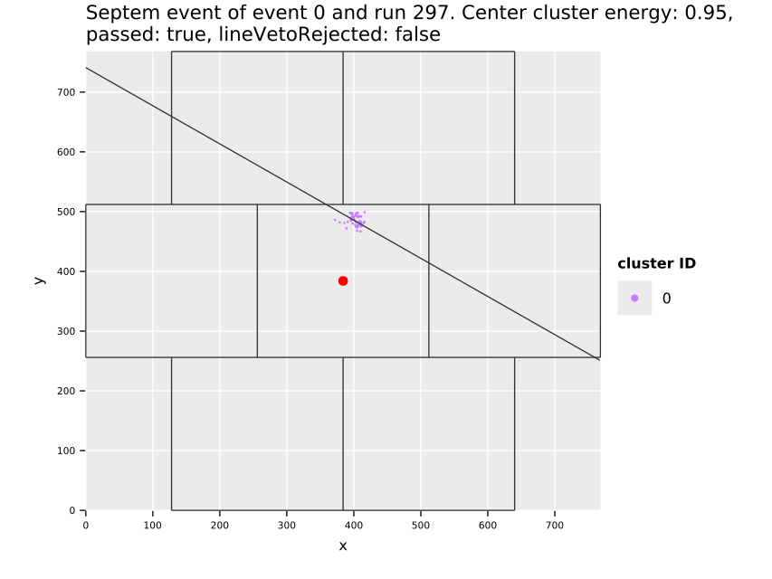
and now with fixed clusters:
    PLOT_SEPTEM_E_CUTOFF=10.0 likelihood \
                          -f ~/CastData/data/DataRuns2018_Reco.h5 \
                          --h5out /tmp/dummy.h5 \
                          --region crAll --cdlYear 2018 \
                          --cdlFile ~/CastData/data/CDL_2019/calibration-cdl-2018.h5 \
                          --septemveto --lineveto --estimateRandomCoinc --estFixedEvent --plotseptem
(Note that the cluster that is chosen can be set using
SEPTEM_FAKE_FIXED_CLUSTER to a different index, by default it just
uses 5).
These events are here:
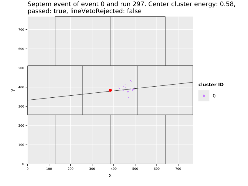
12.5.5.3. TODO Rewrite the whole estimation to a proper program [/] extended
IMPORTANT
That program should call likelihood alone, and likelihood needs to
be rewritten such that it outputs the septem random coincidence (or
real removal) into the H5 output file. Maybe just add a type that
stores the information which we serialize.
With the serialized info about the veto settings we can then
reconstruct in code what is what.
Or possibly better if the output is written to a separate file such that we don't store all the cluster data.
Anyhow, then rewrite the code snippet in the section below that prints the information about the random coincidence rates and creates the plot.
12.5.5.4. Run a whole bunch more cases extended
The below is running now . Still running as of , damn this is slow.
[X]INVESTIGATE PERFORMANCE AFTER IT'S DONE[ ]We should be able to run ~4 (depending on choice even more) in parallel, no?
    import shell, strutils, os

#  let vals = @[1.2, 1.3, 1.4, 1.5, 1.6, 1.7, 1.8, 1.9, 2.0]
#  let vals = @[1.0, 1.1]
let vals = @[  1.0, 1.1, 1.2, 1.3, 1.4, 1.5, 1.6, 1.7, 1.8, 1.9, 2.0  ]
#  let vetoes = @["--lineveto", "--lineveto --estimateRandomCoinc"]
let vetoes = @[  "--septemveto --lineveto", "--septemveto --lineveto --estimateRandomCoinc"  ]

## XXX: ADD CODE DIFFERENTIATING SEPTEM + LINE & LINE ONLY IN NAMES AS WELL!
#  const lineVeto = "lvRegular"
const lineVeto = "lvRegularNoHLC"
let cmd = """
LINE_VETO_KIND=  $#   \
    ECC_LINE_VETO_CUT=  $#   \
    USE_REAL_LAYOUT=true \
    likelihood -f ~/CastData/data/DataRuns2018_Reco.h5 \
    --h5out /t/lhood_2018_crAll_80eff_septem_line_ecc_cutoff_  $#  _  $#  _real_layout  $#  .h5 \
    --region crAll --cdlYear 2018 \
    --cdlFile ~/CastData/data/CDL_2019/calibration-cdl-2018.h5   $#
"""
proc toName  (veto: string  ): string = (  if "estimateRandomCoinc" in veto: "_fake_events" else: ""  )
for val in vals:
  for veto in vetoes:
    let final = cmd % [ lineVeto, $val, $val, lineVeto, toName(veto),
                        $veto ]
    let (res, err) = shellVerbose:
      one:
        cd /tmp
        ($final)
    writeFile  (  "/tmp/logL_output_septem_line_ecc_cutoff_  $#  _  $#  _real_layout  $#  .txt" % [$val, lineVeto, toName(veto)  ], res)
    let outpath = "/home/basti/org/resources/septem_veto_random_coincidences/autoGen/"
    let outfile = "septem_veto_before_after_septem_line_ecc_cutoff_  $#  _  $#  _real_layout  $#  .txt" % [$val, lineVeto, toName(veto)  ]
    copyFile(  "/tmp/septem_veto_before_after.txt", outpath / outfile)
    removeFile(  "/tmp/septem_veto_before_after.txt"  ) #   remove file to not append more and more to file
It has finally finished some time before . Holy moly how slow.
We will keep the generated lhood_* and logL_output_* files in
./../org/resources/septem_veto_random_coincidences/autoGen/ together
with the septem_veto_befor_after_* files.
See the code in one of the next sections for the 'analysis' of this dataset.
12.5.5.5. Number of events removed in real usage extended
[ ]MAYBE EXTEND CODE SNIPPET ABOVE TO ALLOW CHOOSING BETWEEN εcut ANALYSIS AND REAL FRACTIONS
As a reference let's quickly run the code also for the normal use case where we don't do any bootstrapping:
  likelihood \
  -f ~/CastData/data/DataRuns2018_Reco.h5 \
  --h5out /tmp/dummy_real.h5 \
  --region crAll --cdlYear 2018 \
  --cdlFile ~/CastData/data/CDL_2019/calibration-cdl-2018.h5 \
  --septemveto
which results in ./../org/resources/septem_veto_random_coincidences/septem_veto_before_after_only_septem.txt
Next the line veto alone:
  likelihood \
  -f ~/CastData/data/DataRuns2018_Reco.h5 \
  --h5out /tmp/dummy_real.h5 \
  --region crAll --cdlYear 2018 \
  --cdlFile ~/CastData/data/CDL_2019/calibration-cdl-2018.h5 \
  --lineveto
which results in: ./../org/resources/septem_veto_random_coincidences/septem_veto_before_after_only_line.txt
And finally both together:
  likelihood \
  -f ~/CastData/data/DataRuns2018_Reco.h5 \
  --h5out /tmp/dummy_real_2.h5 \
  --region crAll --cdlYear 2018 \
  --cdlFile ~/CastData/data/CDL_2019/calibration-cdl-2018.h5 \
  --septemveto --lineveto
and this finally yields:
./../org/resources/septem_veto_random_coincidences/septem_veto_before_after_septem_line.txt
And further for reference let's compute the fake rate when only using the septem veto (as we have no eccentricity dependence, hence a single value):
  likelihood -f ~/CastData/data/DataRuns2018_Reco.h5 \
  --h5out /tmp/lhood_2018_crAll_80eff_septem_real_layout.h5 \
  --region crAll \
  --cdlYear 2018 \
  --cdlFile ~/CastData/data/CDL_2019/calibration-cdl-2018.h5 \
  --septemveto \
  --estimateRandomCoinc
Run the line veto with new features:
- real septemboard layout
- eccentricity cut off for tracks participating (ecc > 1.6)
    LINE_VETO_KIND=lvRegularNoHLC \
    ECC_LINE_VETO_CUT=1.6 \
    USE_REAL_LAYOUT=true \
    likelihood -f ~/CastData/data/DataRuns2018_Reco.h5 \
    --h5out /tmp/lhood_2018_crAll_80eff_line_ecc_cutof_1.6_real_layout.h5 \
    --region crAll \
    --cdlYear 2018 \
    --cdlFile ~/CastData/data/CDL_2019/calibration-cdl-2018.h5 \
    --lineveto
[ ]WE SHOULD REALLY LOOK INTO RUNNING THE LINE VETO ONLY USING DIFFERENT ε CUTOFFS! -> Then compare the real application with the fake bootstrap application and see if there is a sweet spot in terms of S/N.
Let's calculate the fraction in all cases:
    import strutils
let files = @[  "/home/basti/org/resources/septem_veto_random_coincidences/septem_veto_before_after_only_septem.txt",
              "/home/basti/org/resources/septem_veto_random_coincidences/septem_veto_before_after_only_line.txt",
              "/home/basti/org/resources/septem_veto_random_coincidences/septem_veto_before_after_septem_line.txt",
              "/home/basti/org/resources/septem_veto_random_coincidences/septem_veto_before_after_fake_events_septem.txt",
              "/home/basti/org/resources/septem_veto_random_coincidences/septem_veto_before_after_fake_events_line.txt",
              "/home/basti/org/resources/septem_veto_random_coincidences/septem_veto_before_after_fake_events_septem_line.txt"  ]
proc parseFile  (fname: string  ): float =
  var lines = fname.readFile.strip.splitLines()
  var line = 0
  var numRuns = 0
  var outputs = 0
  #   if file has more than 68 lines, remove everything before, as that means
  #   those were from a previous run
  if lines.len > 68:
    lines = lines  [^68 .. ^1  ]
    doAssert lines.len == 68
  while line < lines.len:
    if lines  [line].len == 0: break
    #   parse input
    #   `  Septem events before: 1069 (L,F) = (false, false)  `
    let input = lines  [line].split(  ':'  )[  1  ].strip.split()[  0  ].parseInt
    #   parse output
    #   `  Septem events after fake cut: 137  `
    inc line
    let output = lines  [line].split(  ':'  )[  1  ].strip.parseInt
    result += output.float / input.float
    outputs += output
    inc numRuns
    inc line
  echo "\tMean output = ", outputs.float / numRuns.float
  result = result / numRuns.float

#   first the predefined files:
for f in files:
  echo "File: ", f
  echo "\tFraction of events left = ", parseFile(f)

#   now all files in our eccentricity cut run directory
const path = "/home/basti/org/resources/septem_veto_random_coincidences/autoGen/"
import std / [os, parseutils, strutils]
import ggplotnim
proc parseEccentricityCutoff  (f: string  ): float =
  let str = "ecc_cutoff_"
  let startIdx = find  (f, str) + str.len
  var res = ""
  let stopIdx = parseUntil(f, res, until = "_", start = startIdx)
  echo res
  result = parseFloat(res)

proc determineType  (f: string  ): string =
  ## I'm sorry for this. :)
  if "only_line_ecc" in f:
    result.add "Line"
  elif "septem_line_ecc" in f:
    result.add "SeptemLine"
  else:
    doAssert false, "What? " & $f
  if "lvRegularNoHLC" in f:
    result.add "lvRegularNoHLC"
  elif "lvRegular" in f:
    result.add "lvRegular"
  else: #   also lvRegularNoHLC, could use else above, but clearer this way. Files
    result.add "lvRegularNoHLC" #   without veto kind are older, therefore no HLC
  if "_fake_events.txt" in f:
    result.add "Fake"
  else:
    result.add "Real"

var df = newDataFrame()
#   walk all files and determine the type
for f in walkFiles(path / "septem_veto_before_after*.txt"  ):
  echo "File: ", f
  let frac = parseFile(f)
  let eccCut = parseEccentricityCutoff(f)
  let typ = determineType(f)
  echo "\tFraction of events left = ", frac
  df.add toDf(  {  "Type" : typ, "ε_cut" : eccCut, "FractionPass" : frac}  )

df.writeCsv(  "/home/basti/org/resources/septem_line_random_coincidences_ecc_cut.csv", precision = 8  )
ggplot(df, aes(  "ε_cut", "FractionPass", color = "Type"  )  ) +
  geom_point() +
  ggtitle(  "Fraction of events passing line veto based on ε cutoff"  ) +
  margin(right = 9  ) +
  ggsave(  "Figs/background/estimateSeptemVetoRandomCoinc/fraction_passing_line_veto_ecc_cut.pdf",
         width = 800, height = 480  )
  #  ggsave("/tmp/fraction_passing_line_veto_ecc_cut.pdf", width = 800, height = 480)

## XXX: we probably don't need the following plot for the real data, as the eccentricity
## cut does not cause anything to get worse at lower values. Real improvement better than
## fake coincidence rate.
#  df = df.spread("Type", "FractionPass").mutate(f{float: "Ratio" ~ `  Real  ` / `  Fake  `})
#  ggplot(df, aes("ε_cut", "Ratio")) +
#    geom_point() +
#    ggtitle("Ratio of fraction of events passing line veto real/fake based on ε cutoff") +
#    #ggsave("Figs/background/estimateSeptemVetoRandomCoinc/ratio_real_fake_fraction_passing_line_veto_ecc_cut.pdf")
#    ggsave("/tmp/ratio_real_fake_fraction_passing_line_veto_ecc_cut.pdf")
(about the first set of files) So about 14.8% in the only septem case and 9.9% in the septem + line veto case.
[ ]MOVE BELOW TO PROPER THESIS PART!
(about the ε cut)

- Investigate significantly lower fake event fraction passing
UPDATE:
The numbers visible in the plot are MUCH LOWER than what we had previously after implementing the line veto alone!!
Let's run with the equivalent of the old parameters:
    LINE_VETO_KIND=lvRegular \
    ECC_LINE_VETO_CUT=1.0 \
    USE_REAL_LAYOUT=false \
    likelihood -f ~/CastData/data/DataRuns2018_Reco.h5 \
    --h5out /t/lhood_2018_crAll_80eff_line_ecc_cutof_1.0_tight_layout_lvRegular.h5 \
    --region crAll --cdlYear 2018 \
    --cdlFile ~/CastData/data/CDL_2019/calibration-cdl-2018.h5 --lineveto --estimateRandomCoinc
-> As it turns out this was a bug in our logic that decides which cluster is of interest to the line veto. We accidentally always deemed it interesting, if the original cluster was on its own… Fixed now.
12.5.6. On the line veto without septem veto extended
When dealing with the line veto without the septem veto there are multiple questions that come up of course.
First of all, what is the cluster that you're actually targeting with our 'line'? The original cluster (OC) that passed lnL or a hypothetical larger cluster that was found during the septem event reconstruction (HLC).
Assuming the former, the next question is whether we want to allow an HLC to veto our OC? In a naive implementation this is precisely what's happening, because in the regular use case of septem veto + line veto, the line veto would never have any effect anymore, as an HLC would almost certainly be vetoed by the septem veto! But without the septem veto, this decision is fully up to the line veto and the question becomes relevant. (we will implement a switch, maybe based on an environment variable or flag)
In the latter case the tricky part is mainly just identifying the correct cluster which to test for in order to find its center. However, this needs to be implemented to avoid the HLC in the above mentioned case. With it done, we then have 3 different ways to do the line veto:
- 'regular' line veto. Every cluster checks the line to the center cluster. Without septem veto this includes HLC checking OC.
- 'regular without HLC' line veto: Lines check the OC, but the HLC is explicitly not considered.
- 'checking the HLC' line veto: In this case all clusters check the center of the HLC.
Thoughts on LvCheckHLC:
- The radii around the new HLC become so large that in practice this won't be a very good idea I think!
- The
lineVetoRejectedpart of the title seems to be "true" in too many cases. What's going on here? See: for example "2882 and run 297" on page 31. Like huh?
My first guess is that the distance calculation is off somehow?
Similar page 33 and probably many more. Even worse is page 34: "event 30 and run 297"!
-> Yeah, as it turns out the problem was just that our
for example "2882 and run 297" on page 31. Like huh?
My first guess is that the distance calculation is off somehow?
Similar page 33 and probably many more. Even worse is page 34: "event 30 and run 297"!
-> Yeah, as it turns out the problem was just that our
inRegionOfInterestcheck had become outdated due to our change of [ ]Select example events for each of the 'line veto kinds' to demonstrate their differences.
OC: Original Cluster (passing lnL cut on center chip)
HCL: Hypothetical Large Cluster (new cluster that OC is part of after
septemboard reco)
Regular:
 is an example event in which we see the "regular" line veto without
using the septem veto. Things to note:
is an example event in which we see the "regular" line veto without
using the septem veto. Things to note:
- the black circle shows the 'radius' of the OC, not the HLC
- the OC is actually part of a HLC
- because of this and because the HLC is a nice track, the event is vetoed, not by the green track, but by the HLC itself!
This wouldn't be a problem if we also used the septem veto, as this
event would already be removed due to the septem veto!
(More plots: 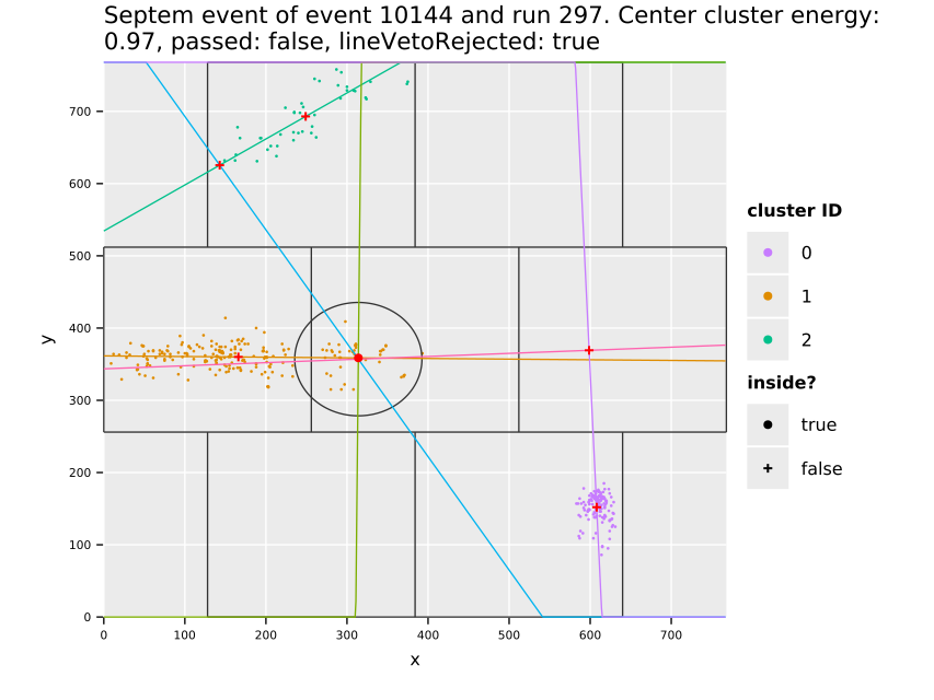 )
)
Regular no HLC:
 The reference cluster to check for is still the regular OC with the
same radius. And again the OC is part of an HLC. However, in contrast
to the 'regular' case, this event is not vetoed. The green and purple
clusters simply don't point at the black circle and the HLC itself is
not considered here. This defines the 'regular no HLC' veto.
The reference cluster to check for is still the regular OC with the
same radius. And again the OC is part of an HLC. However, in contrast
to the 'regular' case, this event is not vetoed. The green and purple
clusters simply don't point at the black circle and the HLC itself is
not considered here. This defines the 'regular no HLC' veto.
 is just an example of an event that proves the method works & a nice
example of a cluster barely hitting the radius of the OC.
On the other hand though this is also a good example for why we should
have an eccentricity cut on those clusters that we use to check for
lines! The green cluster in this second event is not even remotely
eccentric enough and indeed is actually part of the orange track!
(More plots:
is just an example of an event that proves the method works & a nice
example of a cluster barely hitting the radius of the OC.
On the other hand though this is also a good example for why we should
have an eccentricity cut on those clusters that we use to check for
lines! The green cluster in this second event is not even remotely
eccentric enough and indeed is actually part of the orange track!
(More plots: 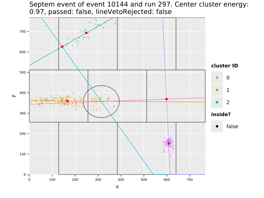 )
)
Check HLC cluster:
 Is an example event where we can see how ridiculous the "check HLC"
veto kind can become. There is a very large cluster that the OC is
actually part of (in red). But because of that the radius is SO
LARGE that it even encapsulates a whole other cluster (that
technically should ideally be part of the 'lower' of the tracks!).
For this reason I don't think this method is particularly useful. In
other events of course it looks more reasonable, but still. There
probably isn't a good way to make this work reliably. In any case
though, for events that are significant in size, they would almost
certainly never pass any lnL cuts anyhow.
(More plots:
Is an example event where we can see how ridiculous the "check HLC"
veto kind can become. There is a very large cluster that the OC is
actually part of (in red). But because of that the radius is SO
LARGE that it even encapsulates a whole other cluster (that
technically should ideally be part of the 'lower' of the tracks!).
For this reason I don't think this method is particularly useful. In
other events of course it looks more reasonable, but still. There
probably isn't a good way to make this work reliably. In any case
though, for events that are significant in size, they would almost
certainly never pass any lnL cuts anyhow.
(More plots: 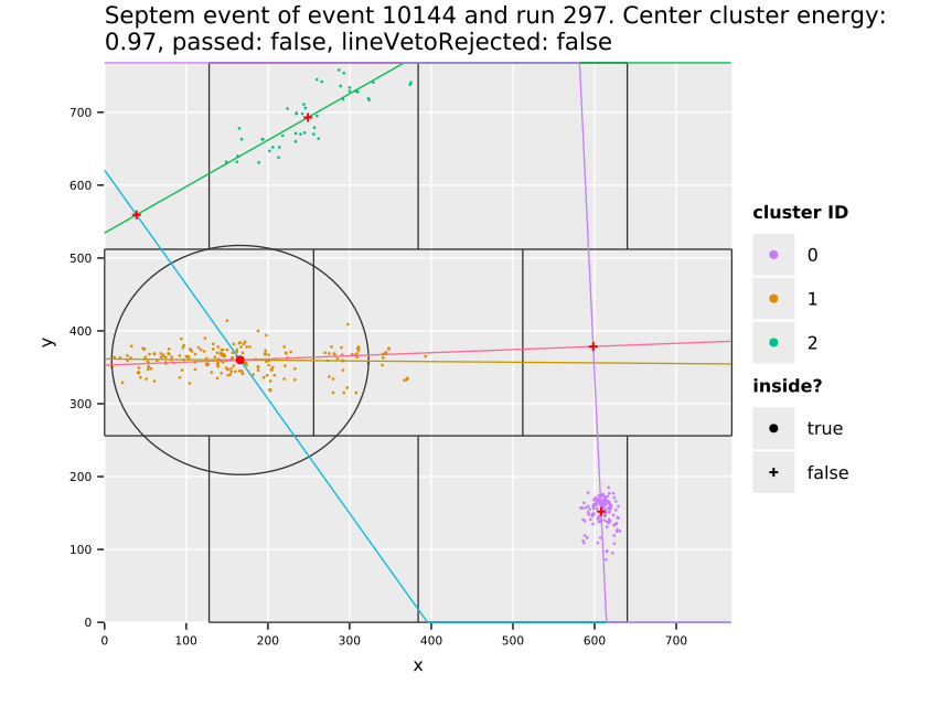 )
)
The following is a broken event. THe purple cluster is not used for line veto. Why? /t/problemevent12435run297.pdf
[X]Implement a cutoff for the eccentricity that a cluster must have in order to partake in the line veto. Currently this can only be set via an environment variable (ECC_LINE_VETO_CUT). A good value is around the 1.4 - 1.6 range I think (anything that rules out most X-ray like clusters!)
12.5.6.1. Note on real septemboard spacing being important extended

is an example event that shows we need to introduce the correct chip
spacing for the line veto. For the septem veto it's not very
important, because the distance is way more important than the angle
of how things match up. But for the line veto it's essential, as can
be seen in that example (note that it uses lvRegularNoHLC and no
septem veto, i.e. that's why the veto is false, despite the purple HLC of
course "hitting" the original cluster)
-> This has been implemented now. Activated (for now) via an
environment variable USE_REAL_LAYOUT.
An example event for the spacing & the eccentricity cutoff is:
file:///home/basti/org/Figs/statusAndProgress/exampleEvents/example_event_with_line_spacing_and_ecc_cutoff.pdf
which was generated using:
    LINE_VETO_KIND=lvRegularNoHLC \
    ECC_LINE_VETO_CUT=1.6 \
    USE_REAL_LAYOUT=true \
    likelihood -f ~/CastData/data/DataRuns2018_Reco.h5 \
    --h5out /tmp/lhood_2018_crAll_80eff_line.h5 \
    --region crAll --cdlYear 2018 \
    --cdlFile ~/CastData/data/CDL_2019/calibration-cdl-2018.h5 \
    --lineveto --plotseptem
and then just extract it from the /plots/septemEvents
directory. Note the definition of the environment variables like this!
12.5.6.2. Outdated: Estimation using subset of outer ring events extended
The text here was written when we were still bootstrapping events only from the subset of event numbers that actually have a cluster that passes lnL on the center chip. This subset is of course biased even on the outer chip. Assuming that center clusters often come with activity on the outer chips, means there are less events representing those cases where there isn't even any activity in the center. This over represents activity on the outer chip.
  likelihood -f ~/CastData/data/DataRuns2018_Reco.h5 \
           --h5out /tmp/lhood_2018_crAll_80eff_septem_fake.h5 \
           --region crAll --cdlYear 2018 \
           --cdlFile ~/CastData/data/CDL_2019/calibration-cdl-2018.h5 \
           --septemveto --estimateRandomCoinc
which writes the file /tmp/septem_fake_veto.txt, which for this case
is found
./../org/resources/septem_veto_random_coincidences/estimates_septem_veto_random_coincidences.txt
Mean value of: 1522.61764706.
From this file the method seems to remove typically a bit less than 500 out of 2000 bootstrapped fake events. This seems to imply a random coincidence rate of almost 25% (or effectively a reduction of further 25% in efficiency / 25% increase in dead time). Pretty scary stuff.
Of course this does not even include the line veto, which will drop it further. Let's run that:
  likelihood -f ~/CastData/data/DataRuns2018_Reco.h5 \
           --h5out /tmp/lhood_2018_crAll_80eff_septem_line_fake.h5 \
           --region crAll --cdlYear 2018 \
           --cdlFile ~/CastData/data/CDL_2019/calibration-cdl-2018.h5 \
           --septemveto --lineveto --estimateRandomCoinc
which generated the following output: ./../org/resources/septem_veto_random_coincidences/estimates_septem_line_veto_random_coincidences.txt
Mean value of: 1373.70588235.
This comes out to a fraction of 68.68% of the events left after running the vetoes on our bootstrapped fake events. Combining it with a software efficiency of ε = 80% the total combined efficiency then would be \(ε_\text{total} = 0.8 · 0.6868 = 0.5494\), so about 55%.
12.5.7. Veto setups of interest [/] extended
[ ]TABLE OF FEATURE, EFFICIENCY, BACKGROUND RATE -> That table essentially motivates looking at different veto setups.[ ]Write a section about a) the motivation behind looking at different setups to begin with and b) show the kind of setups we will be looking at later in the limit part.
As a reference the random coincidence rates of:
- pure septem veto = 0.7841029411764704
- pure line veto = 0.8601764705882353
- septem + line veto = 0.732514705882353
Let's compute the total efficiencies of all the setups we look at.
| limit | name |
|---|---|
| 8.9258e-23 | |
| 8.8516e-23 | _scinti |
| 8.5385e-23 | _scintivetoPercentile0.95fadcvetoPercentile0.95 |
| 7.2889e-23 | _scintivetoPercentile0.95fadcvetoPercentile0.95linevetoPercentile0.95 |
| 7.538e-23 | _scintivetoPercentile0.95fadcvetoPercentile0.95septemvetoPercentile0.95 |
| 7.2365e-23 | _scintivetoPercentile0.95fadcvetoPercentile0.95septemvetoPercentile0.95linevetoPercentile0.95 |
| 8.6007e-23 | _scintivetoPercentile0.99fadcvetoPercentile0.99 |
| 7.3555e-23 | _scintivetoPercentile0.99fadcvetoPercentile0.99linevetoPercentile0.99 |
| 7.5671e-23 | _scintivetoPercentile0.99fadcvetoPercentile0.99septemvetoPercentile0.99 |
| 7.3249e-23 | _scintivetoPercentile0.99fadcvetoPercentile0.99septemvetoPercentile0.99linevetoPercentile0.99 |
| 8.4108e-23 | _scintivetoPercentile0.9fadcvetoPercentile0.9 |
| 7.2315e-23 | _scintivetoPercentile0.9fadcvetoPercentile0.9linevetoPercentile0.9 |
| 7.4109e-23 | _scintivetoPercentile0.9fadcvetoPercentile0.9septemvetoPercentile0.9 |
| 7.1508e-23 | _scintivetoPercentile0.9fadcvetoPercentile0.9septemvetoPercentile0.9linevetoPercentile0.9 |
| \(ε_{\ln\mathcal{L}, \text{eff}}\) | Scinti | FADC | \(ε_{\text{FADC, eff}}\) | Septem | Line | Efficiency | Expected limit (nmc=1000) |
|---|---|---|---|---|---|---|---|
| 0.8 | x | x | - | x | x | 0.8 | 8.9258e-23 |
| 0.8 | o | x | - | x | x | 0.8 | 8.8516e-23 |
| 0.8 | o | o | 0.98 | x | x | 0.784 | 8.6007e-23 |
| 0.8 | o | o | 0.90 | x | x | 0.72 | 8.5385e-23 |
| 0.8 | o | o | 0.80 | x | x | 0.64 | 8.4108e-23 |
| 0.8 | o | o | 0.98 | o | x | 0.61 | 7.5671e-23 |
| 0.8 | o | o | 0.90 | o | x | 0.56 | 7.538e-23 |
| 0.8 | o | o | 0.80 | o | x | 0.50 | 7.4109e-23 |
| 0.8 | o | o | 0.98 | x | o | 0.67 | 7.3555e-23 |
| 0.8 | o | o | 0.90 | x | o | 0.62 | 7.2889e-23 |
| 0.8 | o | o | 0.80 | x | o | 0.55 | 7.2315e-23 |
| 0.8 | o | o | 0.98 | o | o | 0.57 | 7.3249e-23 |
| 0.8 | o | o | 0.90 | o | o | 0.52 | 7.2365e-23 |
| 0.8 | o | o | 0.80 | o | o | 0.47 | 7.1508e-23 |
[ ]ADD THE VERSIONS WE NOW LOOK AT[ ]without FADC[ ]different lnL cut (70% & 90%)
[ ]Maybe introduce a couple of versions with lower lnL software efficiency?[ ]Introduce all setups we care about for the limit calculation, final decision will be done based on which yields the best expected limit.[ ]Have a table with the setups, their background rates (full range) and their efficiencies!
12.6. Background rates of combined vetoes and efficiencies
Having discussed the two main classifiers (likelihood and MLP) as well as all the different possible vetoes, let us now recap. We will look at background rates obtained for different veto setups and corresponding signal efficiencies. In addition, we will compare with fig. 11 – the background clusters left over the entire chip and local background suppression – when using all vetoes.
For a comparison of the background rates achievable in the center \goldArea region using the \lnL method and the MLP, see fig. 36. As already expected from the MLP performance in sec. 12.4.8, it achieves comparable performance at significantly higher signal efficiency. This will be a key feature in the limit calculation to increase the total signal efficiency. The center region does not tell the whole story though, as the background is not homogeneous.

Utilizing all vetoes in addition to the \lnL or MLP classifier alone significantly improves the background rejection over the entire chip. See fig. 37 comparing all remaining X-ray like background cluster centers, without any vetoes and with all vetoes, using the \lnL method at \(ε_{\text{eff}} = \SI{80}{\%}\). While the center background improves, the largest improvements are seen towards the edges and the corners. From a highly non uniform background rate in fig. 37(a), the vetoes produce an almost homogeneous background in 37(b). In total they yield a \(\sim\num{13.5}\) fold reduction in background. Fig. 38 visualizes the improvements by showing the local background suppression, as a factor of the clusters left in each tile over the total number of clusters in the raw data. At closer inspection it is visible that the background improvements are slightly less near the bottom edge of the chip. This is because the spacing to the bottom row of the Septemboard is larger, decreasing the likelihood of detecting a larger cluster.


Tab. 26 shows a comparison of many different possible combinations of classifier, signal efficiency \(ε_{\text{eff}}\), choice of vetoes and total efficiency \(ε_{\text{total}}\). The 'Rate' column is the mean background rate in the range \(\SIrange{0.2}{8}{keV}\) in the center \goldArea region. The \(\ln\mathcal{L}\) produces the lowest background rates, at the cost of low total efficiencies. Generally, many different setups reach into below the \(\SI{1e-5}{keV^{-1}.cm^{-2}.s^{-1}}\) level in the center region, while even large sacrifices in signal efficiency do not yield significantly lower rates. This implies the detector is fundamentally limited at this point in its design. The likely causes being radioactive impurities in the detector material, imperfect cosmic vetoes and lack of better time information in the events. See appendix 31, in particular tab. 33 for the same table with background rates over the entire chip.
The choice for the optimal setup purely based on background rate and total efficiency is difficult, especially because reducing the background to a single number is flawed 36. For this reason we will compute expected limits for each of these setups. The setup yielding the best expected limit will then be used for the calculation of solar tracking candidates and observed limit.
| Classifier | εeff | Scinti | FADC | Septem | Line | εtotal | Rate [\(\si{keV^{-1}.cm^{-2}.s^{-1}}\)] |
|---|---|---|---|---|---|---|---|
| LnL | 0.700 | true | true | true | true | 0.503 | \(\num{ 6.9015(5580)e-06}\) |
| LnL | 0.700 | true | true | false | true | 0.590 | \(\num{ 7.3074(5741)e-06}\) |
| LnL | 0.800 | true | true | true | true | 0.574 | \(\num{ 7.6683(5881)e-06}\) |
| LnL | 0.800 | true | true | false | true | 0.674 | \(\num{ 8.0743(6035)e-06}\) |
| MLP | 0.865 | true | true | true | true | 0.621 | \(\num{ 8.2096(6085)e-06}\) |
| MLP | 0.865 | true | true | false | true | 0.729 | \(\num{ 8.8411(6315)e-06}\) |
| MLP | 0.912 | true | true | true | true | 0.655 | \(\num{ 9.1117(6411)e-06}\) |
| LnL | 0.800 | true | true | true | false | 0.615 | \(\num{ 9.3373(6490)e-06}\) |
| LnL | 0.900 | true | true | true | true | 0.646 | \(\num{ 9.3824(6506)e-06}\) |
| MLP | 0.912 | true | true | false | true | 0.769 | \(\num{ 9.6981(6614)e-06}\) |
| LnL | 0.900 | true | true | false | true | 0.759 | \(\num{ 9.9688(6706)e-06}\) |
| MLP | 0.957 | true | true | true | true | 0.687 | \(\num{1.00139(6721)e-05}\) |
| MLP | 0.957 | true | true | false | true | 0.807 | \(\num{1.05552(6900)e-05}\) |
| MLP | 0.983 | true | true | true | true | 0.706 | \(\num{1.10063(7046)e-05}\) |
| MLP | 0.983 | true | true | false | true | 0.829 | \(\num{1.16378(7245)e-05}\) |
| LnL | 0.800 | true | true | false | false | 0.784 | \(\num{1.55621(8378)e-05}\) |
| MLP | 0.865 | false | false | false | false | 0.865 | \(\num{1.56523(8403)e-05}\) |
| LnL | 0.700 | false | false | false | false | 0.700 | \(\num{1.65545(8641)e-05}\) |
| MLP | 0.912 | false | false | false | false | 0.912 | \(\num{1.74566(8874)e-05}\) |
| LnL | 0.800 | true | false | false | false | 0.800 | \(\num{1.91256(9288)e-05}\) |
| MLP | 0.957 | false | false | false | false | 0.957 | \(\num{2.01631(9537)e-05}\) |
| LnL | 0.800 | false | false | false | false | 0.800 | \(\num{2.06142(9643)e-05}\) |
| MLP | 0.983 | false | false | false | false | 0.983 | \(\num{ 2.3862(1037)e-05}\) |
| LnL | 0.900 | false | false | false | false | 0.900 | \(\num{ 2.7561(1115)e-05}\) |
12.6.1. Generate background rate plots extended
What plots do we want exactly?
    ESCAPE_LATEX=true plotBackgroundRate \
    ~/org/resources/lhood_lnL_17_11_23_septem_fixed/lhood_c18_R2_crAll_sEff_0.8_lnL_scinti_fadc_septem_line_vQ_0.99.h5 \
    ~/org/resources/lhood_lnL_17_11_23_septem_fixed/lhood_c18_R3_crAll_sEff_0.8_lnL_scinti_fadc_septem_line_vQ_0.99.h5 \
    ~/org/resources/lhood_mlp_17_11_23_adam_tanh30_sigmoid_mse_82k/lhood_c18_R2_crAll_sEff_0.95_scinti_fadc_septem_line_mlp_mlp_tanh_sigmoid_MSE_Adam_30_2checkpoint_epoch_82000_loss_0.0249_acc_0.9662_vQ_0.99.h5 \
    ~/org/resources/lhood_mlp_17_11_23_adam_tanh30_sigmoid_mse_82k/lhood_c18_R3_crAll_sEff_0.95_scinti_fadc_septem_line_mlp_mlp_tanh_sigmoid_MSE_Adam_30_2checkpoint_epoch_82000_loss_0.0249_acc_0.9662_vQ_0.99.h5 \
    --names "LnL@80+V" --names "LnL@80+V" \
    --names "MLP@95+V" --names "MLP@95+V" \
    --centerChip 3 \
    --title "Background rate from CAST data, LnL@80% and MLP@95%, all vetoes" \
    --showNumClusters \
    --showTotalTime \
    --topMargin 1.5 \
    --energyDset energyFromCharge \
    --outfile background_rate_crGold_scinti_fadc_septem_line_lnL80_mlp95.pdf \
    --outpath ~/phd/Figs/background/ \
    --useTeX \
    --region crGold \
    --energyMin 0.2 \
    --quiet
#      --applyEfficiencyNormalization \
  plotBackgroundRate \
    ~/org/resources/lhood_mlp_tanh300_outer_chip_training_30_10_23/lhood_c18_R2_crAll_sEff_0.85_mlp_mlp_tanh_sigmoid_MSE_SGD_300_2.h5 \
    ~/org/resources/lhood_mlp_tanh300_outer_chip_training_30_10_23/lhood_c18_R3_crAll_sEff_0.85_mlp_mlp_tanh_sigmoid_MSE_SGD_300_2.h5 \
    ~/org/resources/lhood_mlp_tanh300_outer_chip_training_30_10_23/lhood_c18_R2_crAll_sEff_0.85_scinti_fadc_line_mlp_mlp_tanh_sigmoid_MSE_SGD_300_2_vQ_0.99.h5 \
    ~/org/resources/lhood_mlp_tanh300_outer_chip_training_30_10_23/lhood_c18_R3_crAll_sEff_0.85_scinti_fadc_line_mlp_mlp_tanh_sigmoid_MSE_SGD_300_2_vQ_0.99.h5 \
    ~/org/resources/lhood_mlp_tanh300_outer_chip_training_30_10_23/lhood_c18_R2_crAll_sEff_0.95_mlp_mlp_tanh_sigmoid_MSE_SGD_300_2.h5 \
    ~/org/resources/lhood_mlp_tanh300_outer_chip_training_30_10_23/lhood_c18_R3_crAll_sEff_0.95_mlp_mlp_tanh_sigmoid_MSE_SGD_300_2.h5 \
    ~/org/resources/lhood_mlp_tanh300_outer_chip_training_30_10_23/lhood_c18_R2_crAll_sEff_0.95_scinti_fadc_line_mlp_mlp_tanh_sigmoid_MSE_SGD_300_2_vQ_0.99.h5 \
    ~/org/resources/lhood_mlp_tanh300_outer_chip_training_30_10_23/lhood_c18_R3_crAll_sEff_0.95_scinti_fadc_line_mlp_mlp_tanh_sigmoid_MSE_SGD_300_2_vQ_0.99.h5 \
    ~/org/resources/lhood_limits_automation_with_nn_support/lhood/likelihood_cdl2018_Run2_crAll_lnL.h5 \
    ~/org/resources/lhood_limits_automation_with_nn_support/lhood/likelihood_cdl2018_Run3_crAll_lnL.h5 \
    ~/org/resources/lhood_limits_automation_with_nn_support/lhood/likelihood_cdl2018_Run2_crAll_lnL_scinti_fadc_line_vetoPercentile_0.99.h5 \
    ~/org/resources/lhood_limits_automation_with_nn_support/lhood/likelihood_cdl2018_Run3_crAll_lnL_scinti_fadc_line_vetoPercentile_0.99.h5 \
    --names "MLP@80" --names "MLP@80" \
    --names "MLP8+Sc+F+L" --names "MLP8+Sc+F+L" \
    --names "MLP@91" --names "MLP@91" \
    --names "MLP9+Sc+F+L" --names "MLP9+Sc+F+L" \
    --names "LnL@80" --names "LnL@80" \
    --names "LnL+Sc+F+L" --names "LnL+Sc+F+L" \
    --centerChip 3 \
    --title "Background rate from CAST data" \
    --showNumClusters \
    --showTotalTime \
    --topMargin 1.5 \
    --energyDset energyFromCharge \
    --outfile background_rate_crGold_scinti_fadc_septem_line.pdf \
    --outpath /tmp \
    --useTeX \
    --region crGold \
    --energyMin 0.2 \
    --hideErrors \
    --hidePoints \
    --quiet
#      --applyEfficiencyNormalization \
And now a plot with data 'normalized' by the total signal efficiency. Meaning that if we have e.g. 80% total efficiency, we multiply the total time by that factor, reducing the 'live' time.
This is a decent way to get an idea what veto setting is useful and which isn't (i.e. losing too much efficiency for too little gain in efficiency).
  plotBackgroundRate \
    ~/org/resources/lhood_limits_automation_with_nn_support/lhood/likelihood_cdl2018_Run2_crAll_lnL.h5 \
    ~/org/resources/lhood_limits_automation_with_nn_support/lhood/likelihood_cdl2018_Run3_crAll_lnL.h5 \
    ~/org/resources/lhood_limits_automation_with_nn_support/lhood/likelihood_cdl2018_Run2_crAll_lnL_scinti.h5 \
    ~/org/resources/lhood_limits_automation_with_nn_support/lhood/likelihood_cdl2018_Run3_crAll_lnL_scinti.h5 \
    ~/org/resources/lhood_limits_automation_with_nn_support/lhood/likelihood_cdl2018_Run2_crAll_lnL_scinti_fadc_vetoPercentile_0.99.h5 \
    ~/org/resources/lhood_limits_automation_with_nn_support/lhood/likelihood_cdl2018_Run3_crAll_lnL_scinti_fadc_vetoPercentile_0.99.h5 \
    ~/org/resources/lhood_limits_automation_with_nn_support/lhood/likelihood_cdl2018_Run2_crAll_lnL_scinti_fadc_septem_vetoPercentile_0.99.h5 \
    ~/org/resources/lhood_limits_automation_with_nn_support/lhood/likelihood_cdl2018_Run3_crAll_lnL_scinti_fadc_septem_vetoPercentile_0.99.h5 \
    ~/org/resources/lhood_limits_automation_with_nn_support/lhood/likelihood_cdl2018_Run2_crAll_lnL_scinti_fadc_line_vetoPercentile_0.99.h5 \
    ~/org/resources/lhood_limits_automation_with_nn_support/lhood/likelihood_cdl2018_Run3_crAll_lnL_scinti_fadc_line_vetoPercentile_0.99.h5 \
    ~/org/resources/lhood_limits_automation_with_nn_support/lhood/likelihood_cdl2018_Run2_crAll_lnL_scinti_fadc_septem_line_vetoPercentile_0.99.h5 \
    ~/org/resources/lhood_limits_automation_with_nn_support/lhood/likelihood_cdl2018_Run3_crAll_lnL_scinti_fadc_septem_line_vetoPercentile_0.99.h5 \
    --names "No vetoes" --names "No vetoes" \
    --names "Scinti" --names "Scinti" \
    --names "FADC" --names "FADC" \
    --names "Septem" --names "Septem" \
    --names "noSeptem" --names "noSeptem" \
    --names "Line" --names "Line" \
    --centerChip 3 \
    --title "Background rate from CAST data, incl. scinti, FADC, septem, line veto" \
    --showNumClusters \
    --showTotalTime \
    --topMargin 1.5 \
    --energyDset energyFromCharge \
    --outfile background_rate_crGold_scinti_fadc_septem_line.pdf \
    --outpath /tmp \
    --useTeX \
    --applyEfficiencyNormalization \
    --region crGold \
    --quiet
-> Ok, the above works with, the files all have the logCtx group.
12.6.2. Generate plot of background clusters left over with all vetoes [/] extended
[ ]MAYBE MAKE TEXT FONT WHITE AGAIN?
LnL @ 80% and no vetoes, but using the same zMax as for the all veto case below.
    ESCAPE_LATEX=true plotBackgroundClusters \
    ~/org/resources/lhood_lnL_17_11_23_septem_fixed/lhood_c18_R2_crAll_sEff_0.8_lnL.h5 \
    ~/org/resources/lhood_lnL_17_11_23_septem_fixed/lhood_c18_R3_crAll_sEff_0.8_lnL.h5 \
    --zMax 5 \
    --zMaxSuppression 1000 \
    --title "CAST data, LnL@80%, no vetoes" \
    --outpath ~/phd/Figs/backgroundClusters/ \
    --filterNoisyPixels \
    --energyMin 0.2 --energyMax 12.0 \
    --showGoldRegion \
    --backgroundSuppression \
    --suffix "_lnL80_no_vetoes_zMaxS_1000" \
    --useTikZ
LnL @ 80% and all vetoes:
    ESCAPE_LATEX=true plotBackgroundClusters \
    ~/org/resources/lhood_lnL_17_11_23_septem_fixed/lhood_c18_R2_crAll_sEff_0.8_lnL_scinti_fadc_septem_line_vQ_0.99.h5 \
    ~/org/resources/lhood_lnL_17_11_23_septem_fixed/lhood_c18_R3_crAll_sEff_0.8_lnL_scinti_fadc_septem_line_vQ_0.99.h5 \
    --zMax 5 \
    --zMaxSuppression 1000 \
    --title "CAST data, LnL@80%, all vetoes" \
    --outpath ~/phd/Figs/backgroundClusters/ \
    --filterNoisyPixels \
    --energyMin 0.2 --energyMax 12.0 \
    --showGoldRegion \
    --backgroundSuppression \
    --suffix "_lnL80_all_vetoes_zMaxS_1000" \
    --useTikZ
Background clusters, 95%:
    ESCAPE_LATEX=true plotBackgroundClusters \
    ~/org/resources/lhood_mlp_17_11_23_adam_tanh30_sigmoid_mse_82k/lhood_c18_R2_crAll_sEff_0.95_scinti_fadc_septem_line_mlp_mlp_tanh_sigmoid_MSE_Adam_30_2checkpoint_epoch_82000_loss_0.0249_acc_0.9662_vQ_0.99.h5 \
    ~/org/resources/lhood_mlp_17_11_23_adam_tanh30_sigmoid_mse_82k/lhood_c18_R3_crAll_sEff_0.95_scinti_fadc_septem_line_mlp_mlp_tanh_sigmoid_MSE_Adam_30_2checkpoint_epoch_82000_loss_0.0249_acc_0.9662_vQ_0.99.h5 \
    --zMax 5 \
    --title "Cluster centers CAST data, MLP@95%, all vetoes" \
    --outpath ~/phd/Figs/backgroundClusters/ \
    --filterNoisyPixels \
    --showGoldRegion \
    --energyMin 0.2 --energyMax 12.0 \
    --suffix "_mlp_95_all_vetoes_adam_tanh30_sigmoid_mse_82k" \
    --backgroundSuppression \
    --useTikZ
12.6.3. Generate background rate table extended
Uhhh, excuse this massive wall. I could have written a scrip that reads the files from two directories, but well…
  plotBackgroundRate \
    ~/org/resources/lhood_lnL_17_11_23_septem_fixed/lhood_c18_R2_crAll_sEff_0.8_lnL.h5 \
    ~/org/resources/lhood_lnL_17_11_23_septem_fixed/lhood_c18_R3_crAll_sEff_0.8_lnL.h5 \
    ~/org/resources/lhood_lnL_17_11_23_septem_fixed/lhood_c18_R2_crAll_sEff_0.8_lnL_scinti.h5 \
    ~/org/resources/lhood_lnL_17_11_23_septem_fixed/lhood_c18_R3_crAll_sEff_0.8_lnL_scinti.h5 \
    ~/org/resources/lhood_lnL_17_11_23_septem_fixed/lhood_c18_R2_crAll_sEff_0.8_lnL_scinti_fadc_vQ_0.99.h5 \
    ~/org/resources/lhood_lnL_17_11_23_septem_fixed/lhood_c18_R3_crAll_sEff_0.8_lnL_scinti_fadc_vQ_0.99.h5 \
    ~/org/resources/lhood_lnL_17_11_23_septem_fixed/lhood_c18_R2_crAll_sEff_0.8_lnL_scinti_fadc_septem_vQ_0.99.h5 \
    ~/org/resources/lhood_lnL_17_11_23_septem_fixed/lhood_c18_R3_crAll_sEff_0.8_lnL_scinti_fadc_septem_vQ_0.99.h5 \
    ~/org/resources/lhood_lnL_17_11_23_septem_fixed/lhood_c18_R2_crAll_sEff_0.8_lnL_scinti_fadc_septem_line_vQ_0.99.h5 \
    ~/org/resources/lhood_lnL_17_11_23_septem_fixed/lhood_c18_R3_crAll_sEff_0.8_lnL_scinti_fadc_septem_line_vQ_0.99.h5 \
    ~/org/resources/lhood_lnL_17_11_23_septem_fixed/lhood_c18_R2_crAll_sEff_0.8_lnL_scinti_fadc_line_vQ_0.99.h5 \
    ~/org/resources/lhood_lnL_17_11_23_septem_fixed/lhood_c18_R3_crAll_sEff_0.8_lnL_scinti_fadc_line_vQ_0.99.h5 \
    --names "LnL80" --names "LnL80" \
    --names "LnL80+Sc" --names "LnL80+Sc" \
    --names "LnL80+F" --names "LnL80+F" \
    --names "LnL80+S" --names "LnL80+S" \
    --names "LnL80+SL" --names "LnL80+SL" \
    --names "LnL80+L" --names "LnL80+L" \
    ~/org/resources/lhood_lnL_17_11_23_septem_fixed/lhood_c18_R2_crAll_sEff_0.7_lnL.h5 \
    ~/org/resources/lhood_lnL_17_11_23_septem_fixed/lhood_c18_R3_crAll_sEff_0.7_lnL.h5 \
    ~/org/resources/lhood_lnL_17_11_23_septem_fixed/lhood_c18_R2_crAll_sEff_0.7_lnL_scinti_fadc_line_vQ_0.99.h5 \
    ~/org/resources/lhood_lnL_17_11_23_septem_fixed/lhood_c18_R3_crAll_sEff_0.7_lnL_scinti_fadc_line_vQ_0.99.h5 \
    ~/org/resources/lhood_lnL_17_11_23_septem_fixed/lhood_c18_R2_crAll_sEff_0.7_lnL_scinti_fadc_septem_line_vQ_0.99.h5 \
    ~/org/resources/lhood_lnL_17_11_23_septem_fixed/lhood_c18_R3_crAll_sEff_0.7_lnL_scinti_fadc_septem_line_vQ_0.99.h5 \
    --names "LnL70" --names "LnL70" \
    --names "LnL70+L" --names "LnL70+L" \
    --names "LnL70+S" --names "LnL70+S" \
    ~/org/resources/lhood_lnL_17_11_23_septem_fixed/lhood_c18_R2_crAll_sEff_0.9_lnL.h5 \
    ~/org/resources/lhood_lnL_17_11_23_septem_fixed/lhood_c18_R3_crAll_sEff_0.9_lnL.h5 \
    ~/org/resources/lhood_lnL_17_11_23_septem_fixed/lhood_c18_R2_crAll_sEff_0.9_lnL_scinti_fadc_line_vQ_0.99.h5 \
    ~/org/resources/lhood_lnL_17_11_23_septem_fixed/lhood_c18_R3_crAll_sEff_0.9_lnL_scinti_fadc_line_vQ_0.99.h5 \
    ~/org/resources/lhood_lnL_17_11_23_septem_fixed/lhood_c18_R2_crAll_sEff_0.9_lnL_scinti_fadc_septem_line_vQ_0.99.h5 \
    ~/org/resources/lhood_lnL_17_11_23_septem_fixed/lhood_c18_R3_crAll_sEff_0.9_lnL_scinti_fadc_septem_line_vQ_0.99.h5 \
    --names "LnL90" --names "LnL90" \
    --names "LnL90+L" --names "LnL90+L" \
    --names "LnL90+S" --names "LnL90+S" \
    ~/org/resources/lhood_mlp_17_11_23_adam_tanh30_sigmoid_mse_82k/lhood_c18_R2_crAll_sEff_0.85_mlp_mlp_tanh_sigmoid_MSE_Adam_30_2checkpoint_epoch_82000_loss_0.0249_acc_0.9662.h5 \
    ~/org/resources/lhood_mlp_17_11_23_adam_tanh30_sigmoid_mse_82k/lhood_c18_R3_crAll_sEff_0.85_mlp_mlp_tanh_sigmoid_MSE_Adam_30_2checkpoint_epoch_82000_loss_0.0249_acc_0.9662.h5 \
    ~/org/resources/lhood_mlp_17_11_23_adam_tanh30_sigmoid_mse_82k/lhood_c18_R2_crAll_sEff_0.85_scinti_fadc_line_mlp_mlp_tanh_sigmoid_MSE_Adam_30_2checkpoint_epoch_82000_loss_0.0249_acc_0.9662_vQ_0.99.h5 \
    ~/org/resources/lhood_mlp_17_11_23_adam_tanh30_sigmoid_mse_82k/lhood_c18_R3_crAll_sEff_0.85_scinti_fadc_line_mlp_mlp_tanh_sigmoid_MSE_Adam_30_2checkpoint_epoch_82000_loss_0.0249_acc_0.9662_vQ_0.99.h5 \
    ~/org/resources/lhood_mlp_17_11_23_adam_tanh30_sigmoid_mse_82k/lhood_c18_R2_crAll_sEff_0.85_scinti_fadc_septem_line_mlp_mlp_tanh_sigmoid_MSE_Adam_30_2checkpoint_epoch_82000_loss_0.0249_acc_0.9662_vQ_0.99.h5 \
    ~/org/resources/lhood_mlp_17_11_23_adam_tanh30_sigmoid_mse_82k/lhood_c18_R3_crAll_sEff_0.85_scinti_fadc_septem_line_mlp_mlp_tanh_sigmoid_MSE_Adam_30_2checkpoint_epoch_82000_loss_0.0249_acc_0.9662_vQ_0.99.h5 \
    --names "MLP@85" --names "MLP@85" \
    --names "MLP@85+L" --names "MLP@85+L" \
    --names "MLP@85+S" --names "MLP@85+S" \
    ~/org/resources/lhood_mlp_17_11_23_adam_tanh30_sigmoid_mse_82k/lhood_c18_R2_crAll_sEff_0.9_mlp_mlp_tanh_sigmoid_MSE_Adam_30_2checkpoint_epoch_82000_loss_0.0249_acc_0.9662.h5 \
    ~/org/resources/lhood_mlp_17_11_23_adam_tanh30_sigmoid_mse_82k/lhood_c18_R3_crAll_sEff_0.9_mlp_mlp_tanh_sigmoid_MSE_Adam_30_2checkpoint_epoch_82000_loss_0.0249_acc_0.9662.h5 \
    ~/org/resources/lhood_mlp_17_11_23_adam_tanh30_sigmoid_mse_82k/lhood_c18_R2_crAll_sEff_0.9_scinti_fadc_line_mlp_mlp_tanh_sigmoid_MSE_Adam_30_2checkpoint_epoch_82000_loss_0.0249_acc_0.9662_vQ_0.99.h5 \
    ~/org/resources/lhood_mlp_17_11_23_adam_tanh30_sigmoid_mse_82k/lhood_c18_R3_crAll_sEff_0.9_scinti_fadc_line_mlp_mlp_tanh_sigmoid_MSE_Adam_30_2checkpoint_epoch_82000_loss_0.0249_acc_0.9662_vQ_0.99.h5 \
    ~/org/resources/lhood_mlp_17_11_23_adam_tanh30_sigmoid_mse_82k/lhood_c18_R2_crAll_sEff_0.9_scinti_fadc_septem_line_mlp_mlp_tanh_sigmoid_MSE_Adam_30_2checkpoint_epoch_82000_loss_0.0249_acc_0.9662_vQ_0.99.h5 \
    ~/org/resources/lhood_mlp_17_11_23_adam_tanh30_sigmoid_mse_82k/lhood_c18_R3_crAll_sEff_0.9_scinti_fadc_septem_line_mlp_mlp_tanh_sigmoid_MSE_Adam_30_2checkpoint_epoch_82000_loss_0.0249_acc_0.9662_vQ_0.99.h5 \
    --names "MLP@9" --names "MLP@9" \
    --names "MLP@9+L" --names "MLP@9+L" \
    --names "MLP@9+S" --names "MLP@9+S" \
    ~/org/resources/lhood_mlp_17_11_23_adam_tanh30_sigmoid_mse_82k/lhood_c18_R2_crAll_sEff_0.95_mlp_mlp_tanh_sigmoid_MSE_Adam_30_2checkpoint_epoch_82000_loss_0.0249_acc_0.9662.h5 \
    ~/org/resources/lhood_mlp_17_11_23_adam_tanh30_sigmoid_mse_82k/lhood_c18_R3_crAll_sEff_0.95_mlp_mlp_tanh_sigmoid_MSE_Adam_30_2checkpoint_epoch_82000_loss_0.0249_acc_0.9662.h5 \
    ~/org/resources/lhood_mlp_17_11_23_adam_tanh30_sigmoid_mse_82k/lhood_c18_R2_crAll_sEff_0.95_scinti_fadc_line_mlp_mlp_tanh_sigmoid_MSE_Adam_30_2checkpoint_epoch_82000_loss_0.0249_acc_0.9662_vQ_0.99.h5 \
    ~/org/resources/lhood_mlp_17_11_23_adam_tanh30_sigmoid_mse_82k/lhood_c18_R3_crAll_sEff_0.95_scinti_fadc_line_mlp_mlp_tanh_sigmoid_MSE_Adam_30_2checkpoint_epoch_82000_loss_0.0249_acc_0.9662_vQ_0.99.h5 \
    ~/org/resources/lhood_mlp_17_11_23_adam_tanh30_sigmoid_mse_82k/lhood_c18_R2_crAll_sEff_0.95_scinti_fadc_septem_line_mlp_mlp_tanh_sigmoid_MSE_Adam_30_2checkpoint_epoch_82000_loss_0.0249_acc_0.9662_vQ_0.99.h5 \
    ~/org/resources/lhood_mlp_17_11_23_adam_tanh30_sigmoid_mse_82k/lhood_c18_R3_crAll_sEff_0.95_scinti_fadc_septem_line_mlp_mlp_tanh_sigmoid_MSE_Adam_30_2checkpoint_epoch_82000_loss_0.0249_acc_0.9662_vQ_0.99.h5 \
    --names "MLP@95" --names "MLP@95" \
    --names "MLP@95+L" --names "MLP@95+L" \
    --names "MLP@95+S" --names "MLP@95+S" \
    ~/org/resources/lhood_mlp_17_11_23_adam_tanh30_sigmoid_mse_82k/lhood_c18_R2_crAll_sEff_0.98_mlp_mlp_tanh_sigmoid_MSE_Adam_30_2checkpoint_epoch_82000_loss_0.0249_acc_0.9662.h5 \
    ~/org/resources/lhood_mlp_17_11_23_adam_tanh30_sigmoid_mse_82k/lhood_c18_R3_crAll_sEff_0.98_mlp_mlp_tanh_sigmoid_MSE_Adam_30_2checkpoint_epoch_82000_loss_0.0249_acc_0.9662.h5 \
    ~/org/resources/lhood_mlp_17_11_23_adam_tanh30_sigmoid_mse_82k/lhood_c18_R2_crAll_sEff_0.98_scinti_fadc_line_mlp_mlp_tanh_sigmoid_MSE_Adam_30_2checkpoint_epoch_82000_loss_0.0249_acc_0.9662_vQ_0.99.h5 \
    ~/org/resources/lhood_mlp_17_11_23_adam_tanh30_sigmoid_mse_82k/lhood_c18_R3_crAll_sEff_0.98_scinti_fadc_line_mlp_mlp_tanh_sigmoid_MSE_Adam_30_2checkpoint_epoch_82000_loss_0.0249_acc_0.9662_vQ_0.99.h5 \
    ~/org/resources/lhood_mlp_17_11_23_adam_tanh30_sigmoid_mse_82k/lhood_c18_R2_crAll_sEff_0.98_scinti_fadc_septem_line_mlp_mlp_tanh_sigmoid_MSE_Adam_30_2checkpoint_epoch_82000_loss_0.0249_acc_0.9662_vQ_0.99.h5 \
    ~/org/resources/lhood_mlp_17_11_23_adam_tanh30_sigmoid_mse_82k/lhood_c18_R3_crAll_sEff_0.98_scinti_fadc_septem_line_mlp_mlp_tanh_sigmoid_MSE_Adam_30_2checkpoint_epoch_82000_loss_0.0249_acc_0.9662_vQ_0.99.h5 \
    --names "MLP@98" --names "MLP@98" \
    --names "MLP@98+L" --names "MLP@98+L" \
    --names "MLP@98+S" --names "MLP@98+S" \
    --centerChip 3 \
    --title "Background rate from CAST data, incl. scinti, FADC, septem, line veto" \
    --showNumClusters \
    --showTotalTime \
    --topMargin 1.5 \
    --energyDset energyFromCharge \
    --outfile background_rate_crGold_scinti_fadc_septem_line.pdf \
    --outpath /tmp/ \
    --region crGold \
    --energyMin 0.2 \
    --rateTable ~/phd/resources/background_rate_comparisons.org \
    --noPlot \
    --quiet
Footnotes:
Of course the set of candidates contains background itself. The terminology 'candidate' intends to communicate that each candidate may be a background event or potentially a signal due to axions. But that is part of chapter 13.
In hindsight it seems obvious that a similarly shielded LEMO cable should have been used for the measurements at CAST. Unfortunately, due to lack of experience with electromagnetic interference this was not considered before.
The measurement campaign at the CDL was done in February. However, the weather was nice and sunny most of the week, if I remember correctly. The laboratory has windows towards the south-east. With reasonably cold outside temperatures and sunshine warming the lab in addition to machines and people, opening and closing windows changed the temperature on short time scales, likely significantly contributing to the detector instability. In the extended version of this thesis you'll find a section below this one containing the weather data at the time of the CDL data taking.
Note that similar fits can be performed for the pixel spectra as well. However, as these are not needed for anything further they are only presented in the extended version of the thesis.
The restriction to what is 'visually identifiable' is to avoid the need to fit lines lost in detector resolution and signal to noise ratio. In addition, it avoids overfitting to large numbers of parameters (which brings its own challenges and problems).
We can of course apply the regular energy calibration based on the multiple fits to the CAST calibration data as explained in sec. 11.3. However, due to the very different gas gains observed in the CDL, the applicability is not ideal. Add to that the fact that we know for certain the energy of the clusters in the main fluorescence peak there is simply no need either.
Keep in mind that all energies undergo roughly the same amount of diffusion (aside from the energy dependent absorption length to a lesser extent), so lower energy events are more sparse.
The \(-\ln\mathcal{L}\) values in the distributions give a good idea of why. Roughly speaking the values go from 5 to 20, meaning the actual likelihood values are in the range from \(e^{-5} \approx \num{7e-3}\) to \(e^{-20} \approx \num{2e-9}\)! While 64-bit floating point numbers nowadays in principle provide enough precision for these numbers, human readability is improved. But 32-bit floats would already accrue serious floating point errors due to only about 7 decimal digits accuracy. But even with 64 bit floats, slight changes to the likelihood definition might run into trouble as well.
It's not half the energy as the lines are not evenly spaced in energy.
The only conceptual difference in the techniques is our inclusion of the interpolation between reference distributions in energy.
Due to the rich and long history of artificial neural networks picking "a" or only a few citations is tricky. Amari's work (Amari 1967) was, as far as I'm aware, the first to combine a perceptron with non-linear activation functions and using gradient descent for training. See Schmidhuber's recent overview for a detailed history leading up to modern deep learning (Schmidhuber 2022).
For performance reasons to utilize the parallel nature of GPUs, training and inference of NNs is done in 'mini-batches'. As still only a single loss value is needed for training, the loss is computed as the mean of all losses for each mini-batch element.
The gradients in a neural network are usually computed using 'automatic differentiation' (or 'autograd', 'autodiff'). There are two forms of automatic differentiation: forward mode and reverse mode. These differ by the practical evaluation order of the chain rule. Forward mode computes the chain rule from left-to-right (input to output), while reverse mode computes it from right-to-left (output to input). Computationally these differ in their complexity in terms of the required number of evaluations given N inputs and M outputs. Forward mode computes all M output derivatives for a single input, whereas reverse mode computes all input derivatives for a single output. Thus, forward mode is efficient for cases with few inputs and many outputs, while the opposite is true for reverse mode. Neural networks are classical cases of many inputs to few outputs (scalar loss function!). As such, reverse mode autograd is the standard way to compute the gradients during NN training. In the context it is effectively synonymous with 'backpropagation' (due to its output-to-input evaluation of the chain rule).
The acute reader may wonder why we care less about this for the \(\ln\mathcal{L}\) method. The reason is simply that the effect of gas gain on the three properties used there is comparatively small. But if (almost) all properties are to be used, that is less true.
Generating \(\num{100000}\) fake events of the \cefe photopeak takes around \(\SI{35}{s}\) on a single thread using an AMD Ryzen 9 5950X. The code is not exactly optimized either.
\(σ_T\) would be more appropriate following eq. \eqref{eq:gas_physics:diffusion_after_drift} in sec. 6.3.4.
Note that it is important to consider the transverse standard deviation and not the longitudinal one. Even for an X-ray there will be a short track like signature during production of the primary electrons from the initial photoelectron. This can define the long axis of the cluster in certain cases (depending on gas mixture). Similarly, for background events of cosmic muons the long axis corresponds to the direction of travel while the transverse direction is purely due to the diffusion process.
For example a number provided by Magboltz for the used gas mixture at normal temperature and used chamber pressure. For the CAST gas mixture and settings we start with \(D_T = \SI{660}{μm.cm^{-1/2}}\).
In principle the event generation is the same algorithm as explained previously, but it does not sample from a Pólya for the gas gain, nor compute any cluster properties. Only the conversion point, number of target electrons based on target energy and their positions is simulated. From these electron positions the long and short axes are determined and \(σ_T\) returned.
Initially I tried to compute the gradient using automatic differentiation using dual numbers for the \(D_T\) input and the MC code, but the calculation of the test statistics is effectively independent of the input numbers due to the calculation of the ECDF. As such the derivative information is lost. I didn't manage to come up with a way to compute Cramér-von-Mises based on the actual input numbers directly in a timely manner.
One optimization takes on the order of \(<\SI{30}{s}\) for most runs. But the diffusion parameters are used many times.
This network is considered a "reference" implementation, as it is essentially the simplest ANN layout possible.
libtorch is the C++ library PyTorch is built on.
Yes, only \(\num{30}\) neurons. When using SGD as an optimizer more neurons are useful. With Adam anything more leads to excessive overtraining. Model performance and training time is anyhow better with Adam. Indeed, even a \(\num{10}\) neuron model performs almost as good. The latter is fun, because it allows to write the weight matrices on a piece of paper and almost do a forward pass by hand.
For training X-rays a total of \(\num{500 000}\) events are simulated. For background \(\num{1 000}\) events are randomly selected from each outer chip for each background runs (so \(\num{6 000}\) clusters per background run), totaling \(\num{576 000}\) events. Training and validation is split 50-50.
One could of course interpolate on the cut values itself, but that is less well motivated and harder to cross-check. Predicting a cut value from two known, neighboring energies would likely not work very well.
The number quoted here for \lnL at \(\SI{80}{\%}\) differs slightly from sec. 12.3, because the lower energy range is \(\SI{0.2}{keV}\) here.
A ball park estimate yields a coverage of about \(\SI{35}{°}\) around the zenith. Assuming \(\cos²(θ)\) muons it covers about \(\SI{68}{\%}\) of muons in that axis. With a rate of \(\sim\SI{1}{cm⁻².min⁻¹}\), \(\SI{1125}{h}\) of data with scintillator and \(\SI{4.2}{cm²}\) of active area in front of center GridPix roughly \(\num{194000}\) muons are expected. About \(\num{70000}\) non trivial triggers were recorded. Efficiency of \(\sim\SI{35}{\%}\).
Estimating the number of expected muons for the SiPM is much more difficult, because there is little literature on the actual muon rate at angles close to \(\SI{90}{°}\). The extended version of this thesis contains some calculations, which try to estimate energy distribution and rate under these angles in the detector based on numerically transporting muons from the upper atmosphere to the surface undergoing relativistic effects, changing atmospheric pressures and the related energy loss per distance.
The properties were calculated with
Magboltz using Nimboltz, a Nim interfacer for Magboltz. The code can be found
here:
https://github.com/Vindaar/TimepixAnalysis/Tools/septemboardCastGasNimboltz
Further the numbers used here are for a temperature of \(\SI{26}{°C}\),
slightly above room temperature due to the heating of the Septemboard
itself into the gas.
Of course a properly calibrated scintillator behind the magnet should detect any muons traversing orthogonally. However, it is likely a \(4π\) veto system would be used in a coincidence setup between opposite scintillators. A detector with good time resolution can also detect such events in principle. Despite this, it might be a decent idea to include some lead shielding on the opposite end of future helioscopes to provide some shielding against muons coming from such a direction. In particular a future experiment that tracks the Sun to much higher altitudes will see such muon background significantly more (\(\cos²(θ)\)!).
An alternative could be to attempt to fill in the area between the chips with simulated data based on what is seen at the chip edges. But that is a complex problem. A fun (but possibly questionable) idea would be to train a diffusion model (generative AI) to predict missing data between chips.
In principle this has a small impact on the calculation of the RMS of the cluster, if there is now a large gap between two parts of the 'same' cluster. However, as we don't really rely on the properties too much it is of no real concern. Technically we still calculate the \(\ln\mathcal{L}\) of each cluster, but any cluster passing the \(\ln\mathcal{L}\) cut before being added to a larger cluster almost certainly won't pass it afterwards. The slight bias in the RMS won't change that.
The downside is that DBSCAN is significantly slower, which is part of the reason it is not utilized for the initial reconstruction.
This is roughly the radius of the cluster going by most extended active pixels of the cluster.
Flawed, because a) the background is not homogeneous over the entire chip and the effect of vetoes outside the center region is not visible and b) because the most important range for axion searches is between \(\SIrange{0.5}{5}{keV}\) (depending on the model).