‎

5. Axion helioscopes Theory

As discussed in the previous chapter in section 4.5, stars are strong axion factories. In 1983 Pierre Sikivie proposed (Sikivie 1983, 1985) multiple methods to potentially detect axions, one of these making use of this solar axion production. The fundamental realization is that a transverse magnetic field can act as a means to reconvert axions back into photons, as discussed in sec. 4.4. This allows to design a kind of telescope consisting of a magnet, which tracks the Sun. One expects a small fraction of the axions produced in the Sun to reconvert to photons inside of the magnetic field via the inverse Primakoff effect. These photons will carry the energy of the original particles that produced the axions, namely the energy corresponding to the temperature in the solar core. Some kind of X-ray detector is installed behind the magnet. Ideally, an X-ray telescope can be added to focus any potential X-rays from the full magnet volume onto a smaller area of the detector to massively increase the signal-to-noise ratio.

The first implementation of the helioscope idea was the Rochester-Brookhaven-Florida experiment (Van Bibber et al. 1989; Lazarus et al. 1992). It was followed by the SUMICO experiment in Tokyo (Moriyama et al. 1998; Inoue et al. 2002; Inoue et al. 2008). The third and latest helioscope is the CERN Axion Solar Telescope (CAST), which we will present in more detail in section 5.1. In the final section we will introduce the next generation of axion helioscopes, the International AXion Observatory (IAXO), section 5.2.

5.1. CERN Axion Solar Telescope (CAST)

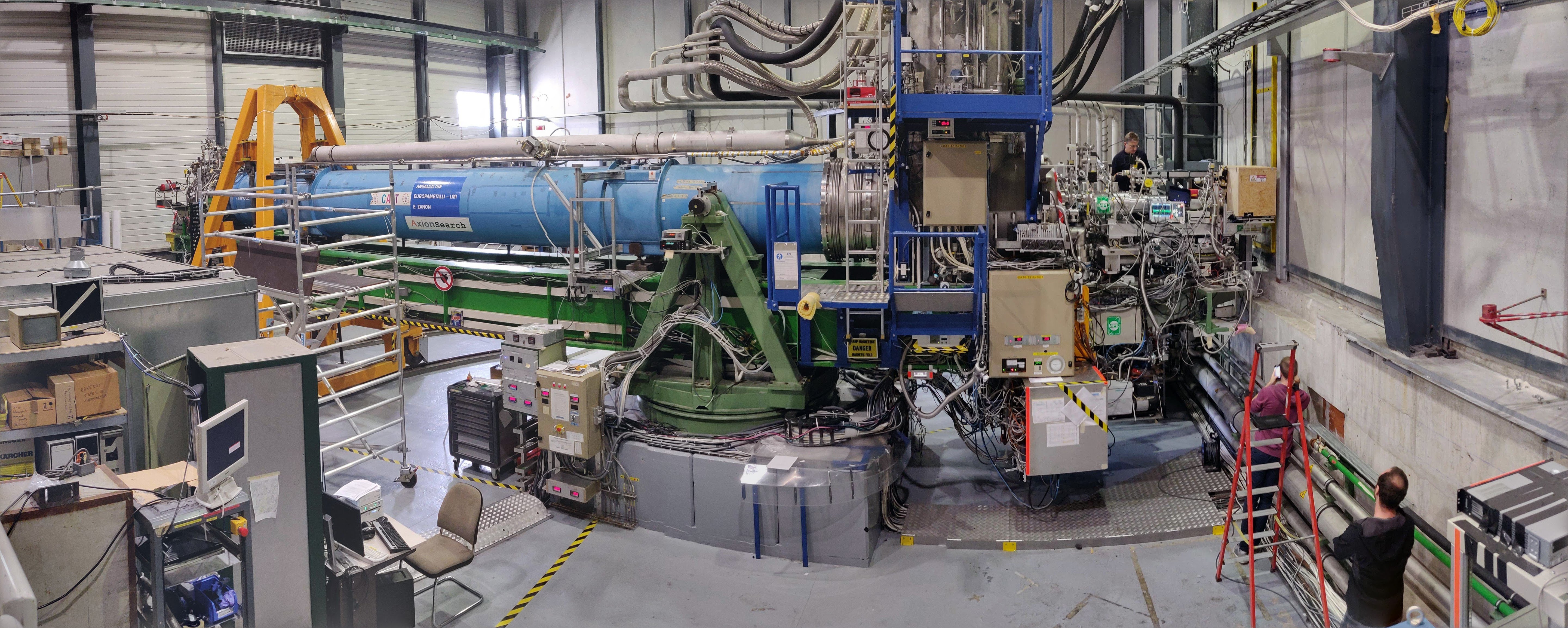
The CERN Axion Solar Telescope (CAST) was proposed in 1999 (Zioutas et al. 1999) and started data taking in 2003 (Zioutas et al. 2005). Fig. 1 shows a panorama view of the experiment in its final year of data taking during some maintenance work.

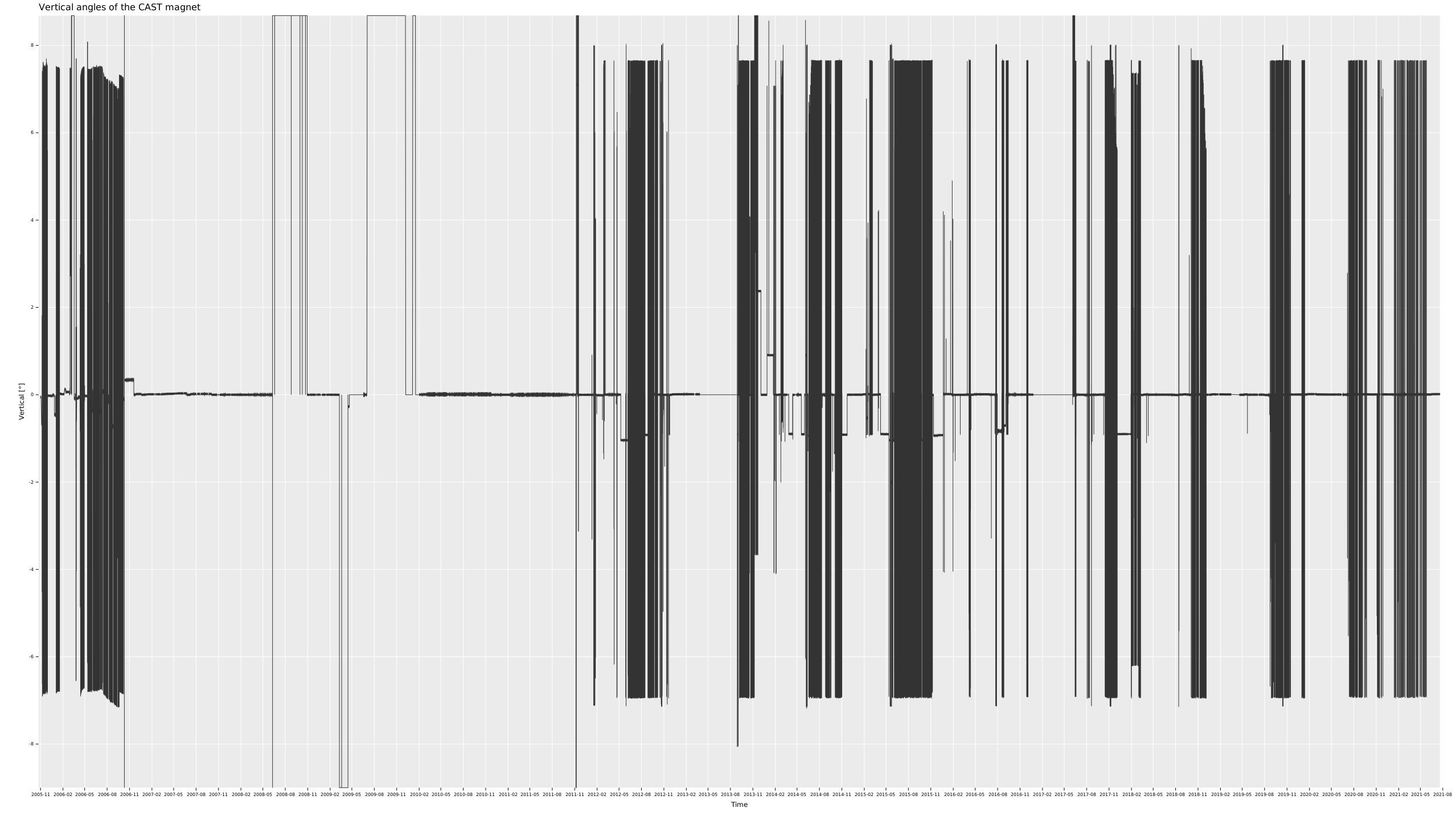
Figure 1: Figure 3: Panorama view of the CAST experiment during some maintenance work.

Using a \(\SI{9.26}{m}\) long Large Hadron Collider (LHC) prototype dipole magnet that was available from the developments for the LHC, CAST features an \(\SI{8.8}{T}\) ¹ strong transverse magnetic field for axion-photon conversion produced by a current of \(\SI{13}{kA}\) in the superconducting \(\ce{Nb Ti}\) wires (Bona et al. 1992) at \(\SI{1.8}{K}\) (Bona et al. 1994). It is placed on a movable platform that allows for solar tracking both during sunrise as well as sunset. The vertical range of movement is about \(\sim\pm\SI{8}{°}\), but practically within \(\sim\SIrange{-7}{7.7}{°}\) ². This range of motion allows for solar tracking of approximately \(\SI{90}{\minute}\) each during sunrise and sunset per day, the exact duration depending on time of the year. Due to the incredibly feeble interactions of axions, solar tracking can already start before sunrise and stop after sunset as they easily traverse through large distances of Earth's mantle.

An LHC dipole magnet has two bores for the two proton beams running in reverse order. Being a prototype magnet it is not bent to the curvature required by the LHC. These two bores have a diameter of \(\SI{4.3}{cm}\). ³ In total then, two bores on each side allow for 4 experiments to be installed at CAST, two for data taking during sunrise and two during sunset.

The first data taking period (often referred to as 'phase I') took place in 2003 for 6 months between May and November and was a pure vacuum run with 3 different detectors. On the side observing during sunset was a Time Projection Chamber (TPC) that covered both bores. On the 'sunrise' side a Micromegas detector (Micromesh Gaseous Detector) and a Charged Coupled Device (CCD) detector were installed. The CCD was further behind a still in place X-ray telescope originally designed as a spare for the ABRIXAS X-ray space telescope (Richter et al. 1995; Friedrich 1998). (Zioutas et al. 2005)

The full first phase I data taking period comprises of data taken in 2003 and 2004 and achieved a best limit of \(g_{aγ} < \SI{8.8e-11}{\GeV^{-1}}\) (Andriamonje et al. 2007).

In what is typically referred to as 'phase II' of the CAST data taking, the magnet was filled with helium as a buffer gas to increase the sensitivity for higher axion masses by inducing an effective photon mass (as mentioned in sec. 4.4.1). First between late 2005 and early 2007 with \(^4\text{He}\). From March 2008 a run with \(^3\text{He}\) was started, which ran until 2011 (Arik et al. 2009; Arik et al. 2015). \(\num{160}\) steps of different gas pressures were used to optimize sensitivity against time per step. In 2012 another \(^4\text{He}\) data run took place (Arik et al. 2015).

From 2013 on the CAST experiment has only run under vacuum configuration (Collaboration and others 2017). Further, the physics scope has been extended to include searches for chameleons (Christoph Krieger 2018; Anastassopoulos et al. 2019, 2015; Baier, n.d.; Cuendis et al. 2019) and axions in the galactic halo via cavity experiments (Cuendis 2021; Melcón et al. 2021; Maroudas 2022; Adair et al. 2022).

A video showing the CAST magnet during a typical solar tracking can be found under the link in this ⁴ footnote.

5.1.1. Generate a plot of the CAST magnet's magnetic field extended

cd ~/CastData/ExternCode/TimepixAnalysis/LogReader/
./cast_log_reader sc -p ../resources/LogFiles/SCLogs/2017_18 -s Version.idx

[ ] SAVE A PLOT
[ ] GET TABLE FROM JAIME's THESIS
[ ] FIND REFERENCE OF JAIME's TABLE

5.1.2. Calculate the maximum tilting angles of the magnet extended

The tilting angles of the CAST magnet are stored (among others, the tracking files also contain angle data, as well as the "angles" file {that existed at some point at least?} ) in the slow control log files.

We'll use our log file parser to parse all the log files between 2016 and

cd ~/CastData/ExternCode/TimepixAnalysis/LogReader/
./cast_log_reader sc -p ../resources/LogFiles/SCLogs -s Version.idx

This yields fig. 2 where we can see that the real angles are between \(\sim\SIrange{-7}{7.7}{°}\).

Figure 2: Figure 4: Vertical angle of the CAST magnet during the data taking discussed in this thesis. The magnet moves in a range of \(\sim\SIrange{-7}{7.7}{°}\) during trackings.

We also have all of the slow control logs in ./../CastData/ExternCode/TimepixAnalysis/resources/LogFiles/AllLogs/logfiles/. Feel free to run the command on this directory. But don't expect amazing performance given the amount of data!

A PNG of the full data in fig. 3 showing the same range as the figure only showing the data taking period discussed in this thesis.

Figure 3: Figure 5: Vertical angle of the CAST magnet during (almost) the entire data taking period from 2005 to end of 2021. Angles go from roughty \(\SI{-7}{°}\) to about \(\SI{7.7}{°}\).

5.1.3. CAST X-ray optics

The first X-ray telescope used at CAST as a focusing optics for the expected axion induced X-ray flux was a Wolter I type X-ray telescope (Wolter 1952) originally built for a proposed German space based X-ray telescope mission, ABRIXAS (Richter et al. 1995; Friedrich 1998). The telescope consists of 27 gold coated parabolic and hyperbolic shells and has a focal length of \(\SI{1.6}{m}\). Due to the small size of the dipole magnet's bores of only \(\SI{43}{mm}\) only a single section of the telescope can be exposed. The telescope is thus placed off-axis from the magnet bore to expose a single mirror section. An image of the mirror system with a rough indication of the exposed section is shown in fig. 4(b).

The telescope is owned by the 'Max Planck Institut für extraterrestrische Physik' in Garching. For that reason it will often be referred to as the 'MPE telescope' in the context of CAST.

The efficiency of the telescope reaches about \(\SI{48}{\%}\) as the peak at around \(\SI{1.5}{keV}\), drops sharply at around \(\SI{2.3}{keV}\) to only about \(\SI{30}{\%}\) up to about \(\SI{7}{keV}\). From there it continues to drop until about \(\SI{5}{\%}\) efficiency at \(\SI{10}{keV}\). The efficiency is shown in a comparison with another telescope in the next section 5.1.4 in fig. 7.

A picture of the telescope installed at CAST behind the magnet on the 'sunrise' side of the magnet is shown in fig. 4(a). ⁵ This telescope was used for the data taking campaign in 2014 and 2015 using a GridPix based detector discussed in (Christoph Krieger 2018) and serves as a comparison for certain aspects in this thesis.

5.1.4. Lawrence Livermore National Laboratory (LLNL) telescope

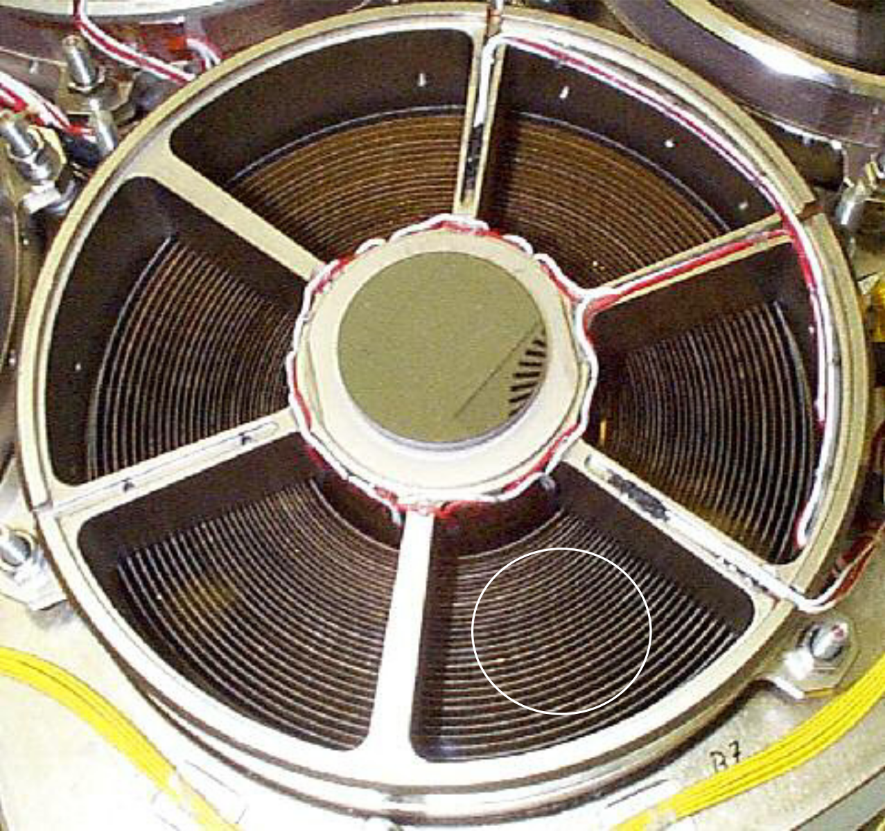
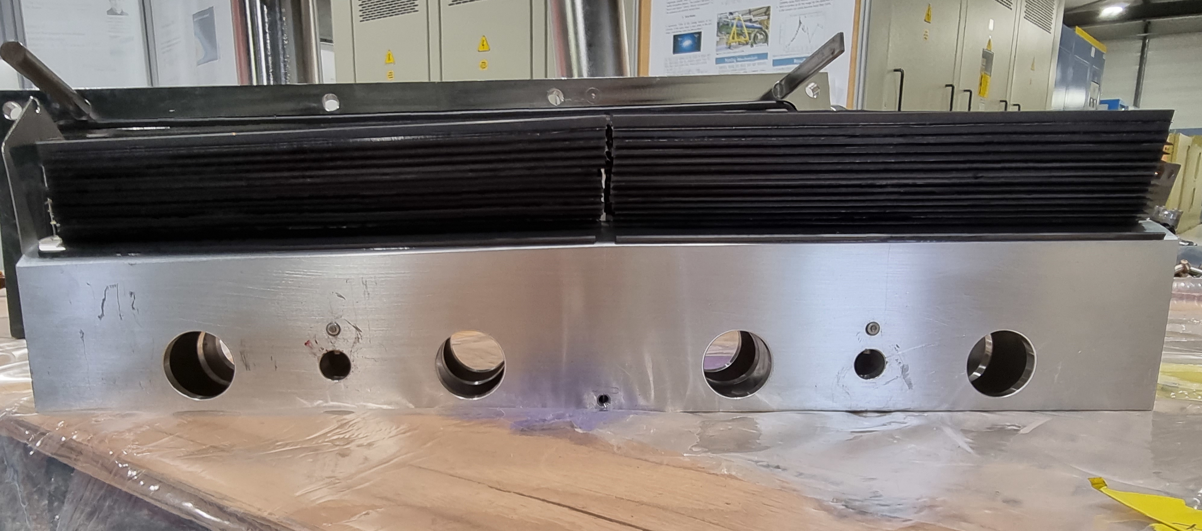
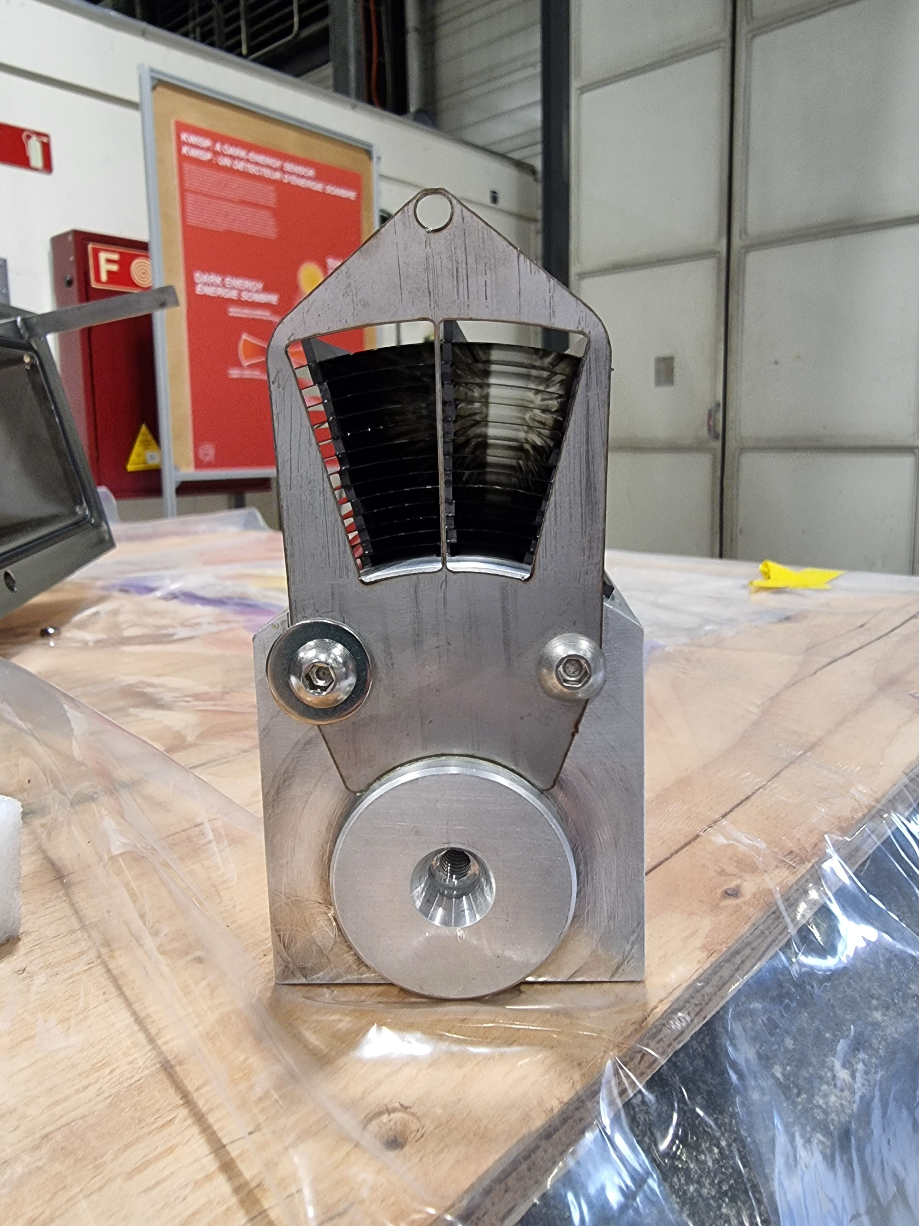
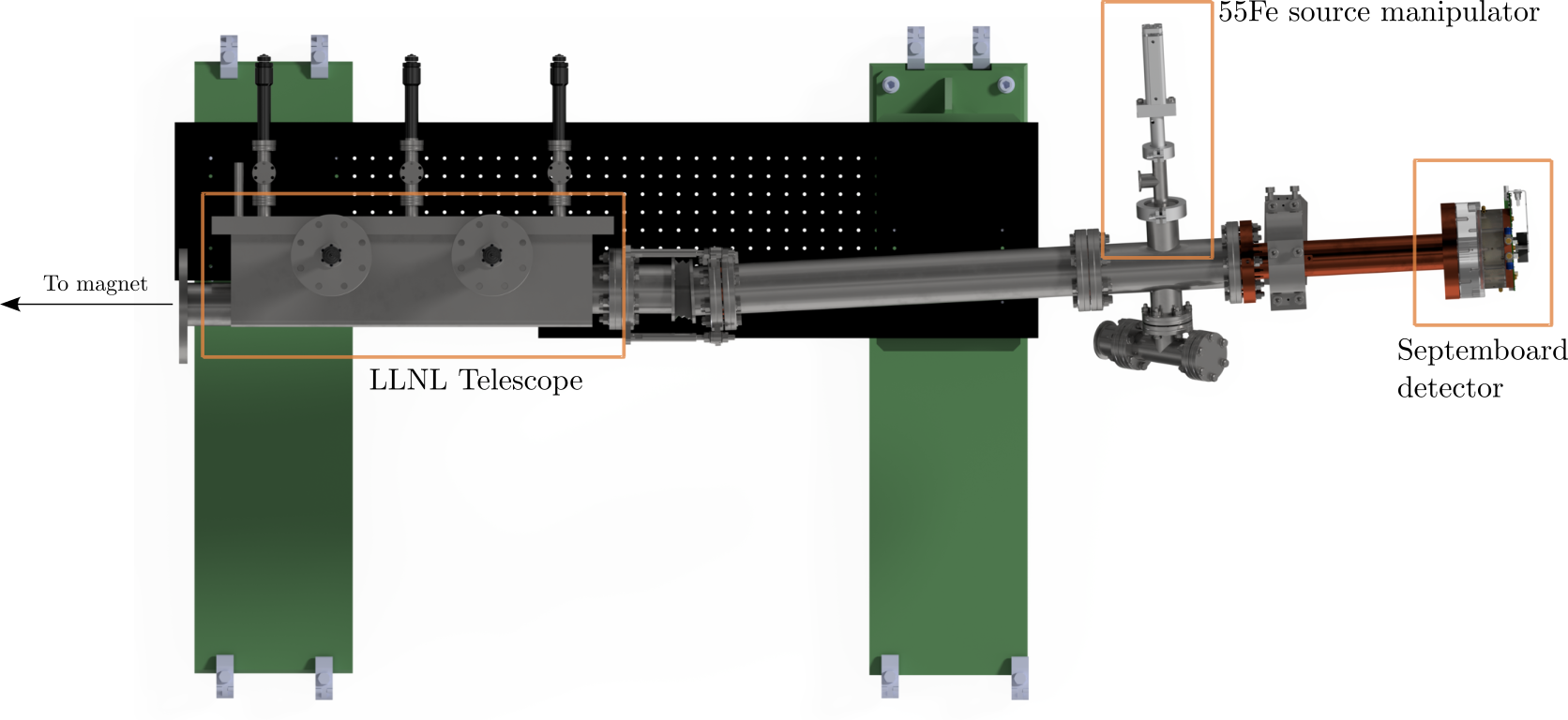
Up to 2014 there was only a single X-ray telescope in use at CAST. In August 2014 a second X-ray optic was installed on the second bore next to the ABRIXAS telescope. This telescope, using technologies originally developed for the space based NuSTAR telescope by NASA (Harrison et al. 2013, 2006; Koglin et al. 2009; Craig et al. 2011; Hailey et al. 2010), was purpose built for axion searches and in particular the CAST experiment. Contrary to the ABRIXAS telescope only a single telescope section of \(\SI{30}{°}\) wide mirrors of the telescope was built as the small bore cannot expose more area anyway. It uses a cone approximation to a Wolter I optic, meaning the hyperbolic and parabolic mirrors are replaced by cone sections (Petre and Serlemitsos 1985). A side view and rear view of the open telescope after decommissioning at CAST are seen in fig. 5. It consists of 13 platinum / carbon coated glass shells in each telescope section, for a total of 26 mirrors. Each mirror uses one of four different depth graded multilayer (see sec. 6.1.2) coating recipes to improve reflectivity over a larger energy and angle range. Further, the focal length was shortened to \(\SI{1.5}{m}\). The telescope section is rotated such that the focal point is pointing away from the other magnet bore to make more space for two detectors side by side. ⁶ This can be seen in the render of the 2017/18 detector setup in fig. 6, seen from the top. The development process of the telescope is documented in the PhD thesis by A. Jakobsen (Jakobsen 2015). (Aznar et al. 2015) gives an overview and shows preliminary results from CAST. The telescope was characterized and calibrated at the PANTER X-ray test facility in Munich.

Figure 6: Figure 6: Render of the setup of the GridPix septemboard detector in 2017/18 showing the LLNL telescope on the left side. The diversion away from the extension of the bore is visible, to have more space for detector installation. The lead shielding and veto scintillator are not shown in the render. Render created by Tobias Schiffer.

This telescope achieves a significantly higher effective area than the ABRIXAS telescope in the energy range between \(\SIrange{2}{3}{keV}\) fig. 7 (relevant for axion searches, compare with fig. #fig:theory:solar_axion_flux:differential_flux). But outside this range the efficiency is comparable or lower.

The precise understanding of the position, size and shape of the focal point as well as the effective area is essential for the limit calculation later in the thesis. In appendix 37 we discuss a raytracing simulation of this telescope. The aim is to simulate the expected distribution of axions from the Sun.

Figure 7: Figure 7: Comparison of the efficiency between the two telescopes, the MPE (ABRIXAS) as the original CAST telescope and the LLNL telescope purpose built for axion searches. The LLNL telescope has superior efficiency in the energy range where the axion flux is assumed to dominate, but falls off sharper at high energies. The data for the LLNL telescope is extracted from fig. 3 in llnl_telescope_first_cast_results, whereas for the ABRIXAS telescope it is extracted from the red line in fig. 4 of CAST_telescope_ccd.

5.1.4.1. Generate effective area plot for LLNL and MPE telescopes `[/]` extended

We'll now create the comparison plot of the effective areas for the two X-ray telescopes used at CAST.

For the MPE telescope: As mentioned in the caption of the figure above, the data for the MPE telescope is extracted from fig. 4 of (Kuster et al. 2007), also found here . This is done using ./code/other/extractDataFromPlot.nim using a simplified version of fig. 4 as an input (i.e. crop the plot to exactly the area of the actual plot and remove any lines that are not the data to be extracted. This plot looks like mpe_xray_telescope_cast_effective_area_cropped_no_axes.png .

Then run

./extractDataFromPlot \
    -f ~/phd/resources/MPE/mpe_xray_telescope_cast_effective_area_cropped_no_axes.png \
    --xLow 0.305 --xHigh 10.0 \
    --yLow 0.0 --yHigh 8.0

which produces a plot from the extracted data and writes a CSV file, which

[X] Make sure to add the effective area files to a resources directory of the thesis repo!
[ ] Ask Jaime if this really looks sensible, because to me it does not! That's barely better than the MPE telescope…

import ggplotnim, ggplotnim/ggplot_sdl2
import unchained
const mpe = "~/phd/resources/MPE/mpe_xray_telescope_cast_effective_area.csv"
const llnl = "~/phd/resources/LLNL/EffectiveArea.txt"
let dfMpe = readCsv(mpe)
let dfLLNL = readCsv(llnl, sep = ' ')
  .rename(f{"Energy[keV]" <- "E(keV)"},
          f{"EffectiveArea[cm²]" <- "Area(cm^2)"})
let df = bind_rows([("MPE", dfMpe), ("LLNL", dfLLNL)], "Telescope")
const areaBore = (4.3.cm / 2.0)^2 * π ## Area of the CAST bore in cm²
ggplot(df, aes("Energy[keV]", "EffectiveArea[cm²]", color = "Telescope")) +
  geom_line() +
  xlab(r"Energy [\si{keV}]") + ylab(r"EffectiveArea [\si{cm^2}]") +
  scale_y_continuous(secAxis = secAxis(f{1.0 / areaBore.float}, name = r"Transmission [\si{\%}]")) +
  legendPosition(0.83, -0.2) +
  themeLatex(fWidth = 0.9, width = 600, baseTheme = singlePlot) + 
  ggshow("~/phd/Figs/telescopes/effective_area_mpe_llnl.pdf", useTeX = true, standalone = true)

5.1.5. Best limits set by CAST

In the many years of data taking and countless detectors taking data at the CAST experiment, it has put the most stringent limits on different coupling constants over the years.

Specifically, CAST sets the current best helioscope limits on the:

Axion-photon coupling \(g_{aγ}\)
Axion-electron coupling \(g_{ae}\)
Chameleon-photon coupling \(β_γ\)

For the axion-photon coupling the best limit is from (Collaboration and others 2017) in 2017 based on the full Micromegas dataset including the data behind the LLNL telescope and constricts the coupling to \(g_{aγ} < \SI{6.6e-11}{\GeV^{-1}}\).

For the axion-electron coupling the best limit is still from 2013 in (Barth et al. 2013) using the theoretical calculations for an expected solar axion flux done by J. Redondo in (Redondo 2013) for a limit on the product of the axion-electron and axion-photon coupling of \(g_{ae} · g_{aγ} < \SI{8.1e-23}{\GeV^{-1}}\). The limit calculation was based on data taken in CAST phase I in 2003 - 2005 with a pn-CCD detector behind the MPE telescope.

CAST was also used to set a limit on the hypothetical chameleon particle. The best current limit on the chameleon-photon coupling \(β_γ\) is based on a single GridPix based detector with data taken in 2014 and 2015 by C. Krieger in (Christoph Krieger 2018; Anastassopoulos et al. 2019), limiting the coupling to \(β_γ < \num{5.74e10}\), which is the first limit below the solar luminosity bound.

5.2. International AXion Observatory (IAXO)

Barring a revolution in detector development or a lucky find of a non QCD axion, the CAST experiment was unlikely to detect any signals. A fourth generation axion helioscope to possibly reach towards the QCD band in the mass-coupling constant phase space is a natural idea.

The first proposal for a next generation axion helioscope was published in 2011 (Irastorza et al. 2011), with the name International AXion Observatory (IAXO) first appearing in 2013 (Vogel et al. 2013). A conceptual design report (CDR) was further published in 2014 (Armengaud et al. 2014).

The proposed experiment is supposed to have a total magnet length of \(\SI{25}{m}\) length with eight \(\SI{60}{cm}\) bores with an average transverse magnetic field of \(\SI{2.5}{T}\) ⁷. With a cryostat and magnet design specifically built for the experiment, much larger tilting angles of the magnet of about \(\pm\SI{25}{°}\) are proposed to allow for solar tracking for \(\SI{12}{\hour}\) per day for a 1:1 data split between tracking and background data. (Armengaud et al. 2014)

In (Irastorza et al. 2011) a 'figure of merit' (FOM) is introduced to quantify the improvements possible by IAXO over CAST, defined by

\[ f = f_M f_{\text{DO}} f_T = (B² L² A)_M \left(\frac{ε_d ε_o}{\sqrt{b a}}\right)_{\text{DO}} (\sqrt{ε_t t})_T \]

which is split into individual FOMs for the magnet \(f_M\), the detector and optics \(f_{\text{DO}}\) and the total tracking time \(f_T\) (\(B\): magnetic field, \(L\): magnet length, \(A\): total bore area of all bores, \(ε_d\): detector efficiency, \(ε_o\): X-ray optic efficiency, \(b\): background in counts per area and time, \(a\): area of the X-ray optic focal spot, \(ε_t\): data taking efficiency, \(t\): total solar tracking time). The biggest improvements would come from the magnet FOM (MFOM), due to the much larger magnet volume. Compared to the CAST MFOM \(f_{M,\text{CAST}} = \SI{19.3}{T^2.m^4}\) IAXO would achieve a relative improvement of \(f_{M,\text{CAST}} / f_{M,\text{IAXO}} \approx 300\) with its \(f_{M,\text{IAXO}} = \SI{5654.9}{T^2.m^4}\). As the number of expected counts in a helioscope scales with \(g^4\) ⁸, the figure of merit directly relates possible limits of a helioscope in case of a non-detection. The aspirational target for IAXO would be a full \(f_{\text{CAST}} / f_{\text{IAXO}} > \num{10000}\) for a possible improvement on \(g\) bounds by an order of magnitude.

A schematic of the proposed design can be seen in fig. 8(a). Given the comparatively large budget requirements for such an experiment, a compromise was envisioned to prove the required technologies, in particular the magnet design. This intermediate experiment called BabyIAXO will be discussed in the next section, 5.2.1.

5.2.1. BabyIAXO

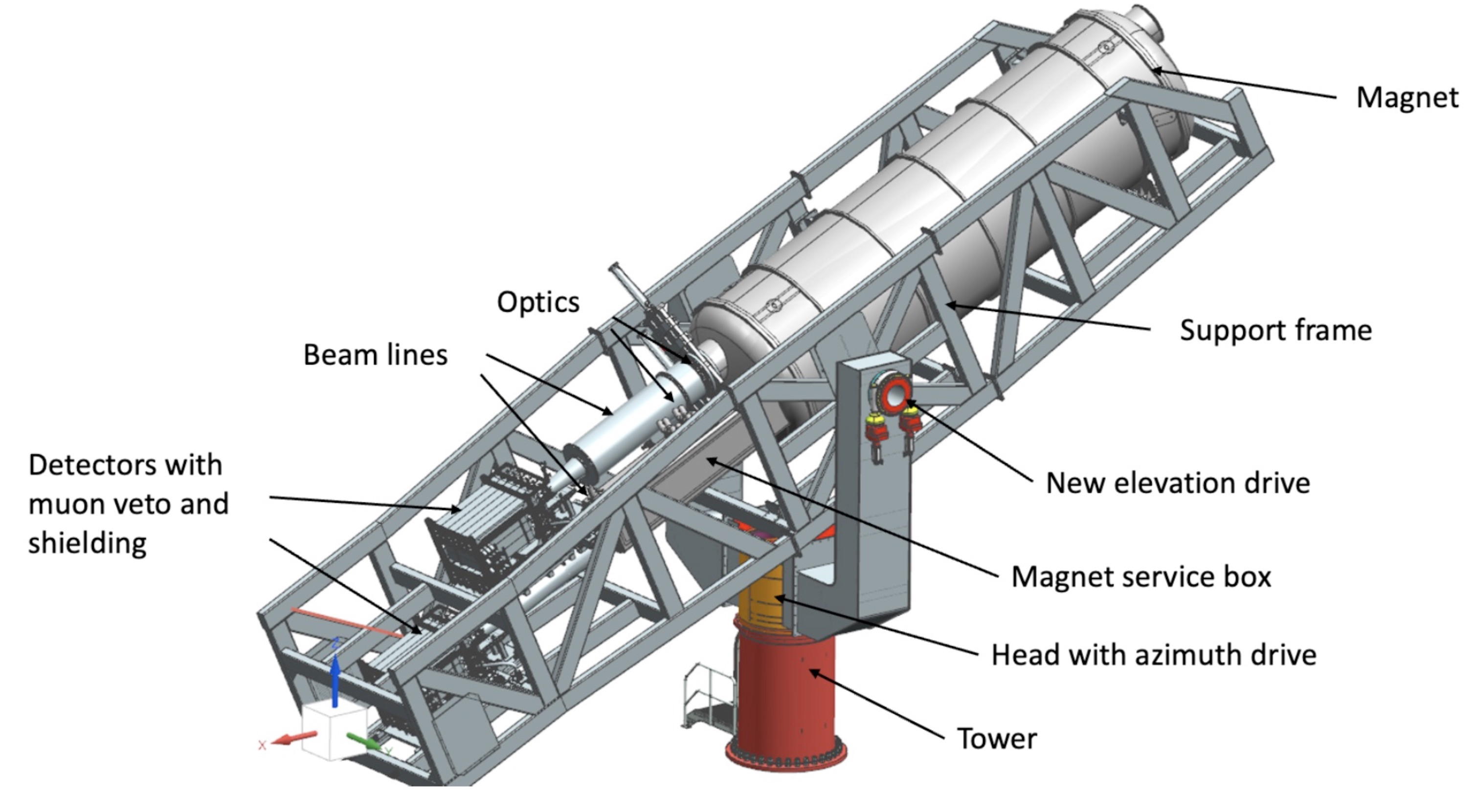
The major difference between full grown IAXO and BabyIAXO is restricting the setup to 2 bores instead of 8 with a magnet length of only \(\SI{10}{m}\) to prove the magnet design works, before building a larger version of said design. Since the first conceptual design of IAXO (Armengaud et al. 2014) the bore diameter for the two bores of BabyIAXO has increased from \(\SI{60}{cm}\) to \(\SI{70}{cm}\). (Collaboration et al. 2021)

The BabyIAXO design was approved by the 'Deutsches Elektronen-Synchrotron' (DESY) for construction onsite. The project has suffered multiple delays most notably due to the magnet construction. First COVID19 due to its severe effects on supply chains and in 2022 the horrific Russian invasion of Ukraine have caused multi year delays. The latter in particular was problematic as the only two companies being able to supply the type of superconducting cable needed for the magnet are from Russia. The magnet situation is still in flow as of writing this thesis.

For the two bores two different X-ray telescopes are planned to be operated. One bore will be used with a flight spare of the XMM-Newton X-ray satellite mission with a focal length of \(\SI{7.5}{m}\). The second bore would receive a custom built X-ray optic based on a hybrid design of a NuSTAR-like optic for the inner part – similar to the LLNL telescope introduced in sec. 5.1.4 (just as a full telescope) – and a cold slumped glass design following (Civitani et al. 2016) for the outer part. This optic would have a focal length of only \(\SI{5}{m}\).

An annotaded schematic of the BabyIAXO design can be seen in fig. 8(b). The magnet figure of merit for BabyIAXO is aimed at being at least a factor 10 higher than for CAST, with (Collaboration et al. 2021) listing values between \(\SIrange{232}{326}{T^2.m^4}\) depending on how it is calculated.

Footnotes:

The magnetic field of \(\SI{8.8}{T}\) corresponds to the actual field at which the magnet was operated at CAST, as taken from the magnet slow control data.

These numbers are from CAST's slow control logs. See the extended thesis.

There is some confusion about the diameter and length of the magnet. The original CAST proposal (Zioutas et al. 1999) talks about the prototype dipole magnets as having a bore diameter of \(\SI{42.5}{mm}\) and a length of \(\SI{9.25}{m}\). However, every CAST publication afterwards uses the numbers \(\SI{43}{mm}\) and \(\SI{9.26}{m}\). Digging into references about the prototype dipole magnets is inconclusive. For better compatibility with all other CAST related publications, we will use the same \(\SI{43}{mm}\) and \(\SI{9.26}{m}\) values in this thesis. Furthermore, measurements were done indicating values around \(\SI{43}{mm}\).

⁴

https://www.youtube.com/watch?v=XY2lFDXz8aQ

⁵

See appendix section 20.1 for a schematic of the common terminology like 'sunrise' used at CAST.

⁶

Because this telescope only consists of one section, its focal point is 'parallel' to the magnet bore. In a full Wolter I like optic the focal point is exactly behind the center of the optic. With only a portion of a telescope this implies an offset. Further, the telescope is not actually rotated exactly \(\SI{90}{°}\) to move the focal spot perfectly parallel to the two bores, but only about \(\SI{76}{°}\).

⁷

Due to the envisioned toroidal magnet design and much larger diameter, the magnetic field inside such a bore would not be as homogeneous as in the LHC dipole magnets. The peak field would be about \(\SI{5.4}{T}\). This also means a correct \(f_M\) calculation for IAXO must take into account the actual magnetic field map.

⁸

\(g⁴\) is a placeholder for \(g⁴_{aγ}\) or \(g²_{aγ}·g²_{ae}\). The flux scales with this product as explained in sec. 4.7 due to axion production and reconversion happening via \(g²\) each.

Click on any heading marked 'extended' to open it