7. Septemboard detector Detector
With the theoretical aspects of gaseous detectors out of the way, in sec. 7.1 we will introduce the 'Micromegas' type of gaseous detector. Micromegas can be read out in different ways. One option is the Timepix ASIC, sec. 7.2, by way of the 'GridPix', sec. 7.3.
The GridPix detector in use in the 2014 / 2015 CAST data taking campaign, to be presented in section 7.4, had a few significant drawbacks for more sensitive searches. In particular for searches at low energies \(\lesssim\SI{2}{\keV}\) and searches requiring low backgrounds over larger areas on the chip (for example the chameleon search done in (Christoph Krieger 2018)). For this reason a new detector was built in an attempt to improve each shortcoming of the detector.
We introduce the 'Septemboard' detector with a basic overview in section 7.5. From there we continue looking at each of the new detector features motivating their addition. All detector upgrades were done to alleviate one or more of the old detector's drawbacks. For each new detector feature we will highlight the aspects it is intended to improve on.
Section 7.7 introduces two new scintillators as vetoes. These require the addition of an external shutter for the Timepix, which is realized by usage of a flash ADC (FADC), see section 7.8. Further, an independent but extremely important addition is the replacement of the Mylar window by a silicon nitride window, section 7.9. Another aspect is the addition of 6 GridPixes around the central GridPix, the 'Septemboard' introduced in section 7.10. Due to the additional heat produced by 6 more GridPix, a water cooling system is used, sec. 7.11. Lastly, in sec. 7.12 we will also discuss the combined detection efficiency of this detector.
7.1. Micromegas working principle
\textbf{Micro} \textbf{Me}sh \textbf{Ga}seous \textbf{S}tructures (Micromegas) are a kind of \textbf{M}icro\textbf{p}attern \textbf{G}aseous \textbf{D}etectors (MPGDs) first introduced in 1996 (Giomataris et al. 1996; Giomataris 1998). The modern Micromegas is the Microbulk Micromegas (Andriamonje et al. 2010).
Interestingly, the name Micromegas is based on the novella Micromégas by Voltaire published in 1752 (Voltaire 1752), an early example of a science fiction story. (Giomataris et al. 1996)
These detectors are – as the name implies – gaseous detectors containing a 'micro mesh'. In the most basic form they are a made of a closed detector volume that is filled with a suitable gas, allowing for ionization (often argon based gas mixtures are used; xenon based detectors for axion helioscopes are in the prototype phase). The volume is split into two different sections, a large drift volume typically \(\mathcal{O}(\text{few }\si{cm})\) and an amplification region, sized \(\mathcal{O}(\SIrange{50}{100}{μm})\). At the top of the volume is a cathode to apply an electric field. Below the mesh is the readout area at the bottom of the volume. In standard Micromegas detectors, strips or pads are used as a readout. The electric field in the drift region is strong enough to avoid recombination of the created electron-ion pairs and to provide reasonably fast drift velocities \(\mathcal{O}(\si{cm.μs⁻¹})\). The amplification gap on the other hand is precisely used to multiply the primary electrons using an avalanche effect. Thus, the electric field reaches values of \(\mathcal{O}(\SI{50}{kV.cm⁻¹})\). These drift and amplification volumes are achieved by an electric field between a cathode and the mesh as well as the mesh and the readout area.
Fig. 1 shows a schematic for the general working principle of such detectors

7.2. Timepix ASIC
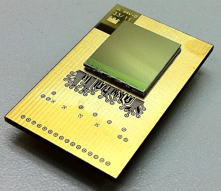
The Timepix ASIC (Application Specific Integrated Circuit) is a \(256 × 256\) pixel ASIC with each pixel \(\num{55}·\SI{55}{μm^2}\) in size. It is based on the Medipix ASIC, developed for medical imaging applications by the Medipix Collaboration (Llopart et al. 2002). The pixels are distributed over an active area of \(\num{1.41}\times\SI{1.41}{\cm^2}\). Each pixel contains a charge sensitive amplifier, a single threshold discriminator and a \(\SI{14}{bit}\) pseudo random counting logic. It requires use of an external clock, in the range of \(\SIrange{10}{150}{MHz}\), with \(\SI{40}{MHz}\) being the clock frequency used for the applications in this thesis. (Llopart Cudie 2007; Llopart et al. 2007; Llopart and Poikela 2006) A good overview of the Timepix is also given in (Lupberger 2016). A picture of a Timepix ASIC is shown in fig. 2(a).
The Timepix uses a shutter based readout, either with a fixed shutter time or using an external trigger to close a frame. After the shutter is closed in the Timepix, the readout is performed during which the detector is insensitive. Each pixel further can work in four different modes:
- hit counting mode / single hit mode
- simply counts the number of times the threshold of a pixel was crossed (or whether a pixel was activated once in single hit mode).
- \textbf{T}ime \textbf{o}ver \textbf{T}hreshold (ToT)
- In the ToT mode the counter of a pixel will count the number of clock cycles that the charge on the pixel exceeds the set threshold, which is set by an \(\SI{8}{bit}\) \textbf{D}igital to \textbf{A}nalog \textbf{C}onverter (DAC) while the shutter is open. ToT is equivalent to the collected charge of each pixel.
- \textbf{T}ime \textbf{o}f \textbf{A}rrival (ToA)
- The ToA mode records the number of clock cycles from the first time the pixel's threshold is exceeded to the end of the shutter window. Thus, it allows to calculate the time at which the pixel first crossed the threshold.
In the context of this thesis only the ToT mode was used.
7.2.1. Timepix3
The Timepix3 is the successor of the Timepix. (Poikela et al. 2014; Llopart and Poikela 2015) It is generally similar to the Timepix, but would provide 3 important advantages if used in a gaseous detector for the applications in this thesis:
- clock rates of up to \SI{300}{MHz} for higher possible data rates (less interesting for data taking in an axion helioscope)
- a stream based data readout. This means no fixed shutter times and no dead time during readout. Instead data is sent out when it is recorded in parallel.
- each pixel can record ToT and ToA information at the same time. This allows to record the charge recorded by a pixel as well as the time it was activated, yielding 3D event reconstruction with precise charge information.
An open source readout was developed by the University of Bonn and is available under (Gruber et al. 2023) 1. A gaseous detector based on this is currently in the prototyping phase, see the upcoming (Schiffer 2024).
7.3. GridPix
First experiments of combining a Micromegas with a Timepix readout were done in 2005 (Campbell et al. 2005) by using classical approaches to place a micromesh on top of the Timepix, at the time still called TimePixGrid. While this worked in principle, it showed a Moiré pattern, due to slight misalignment between the holes of the micromesh and the pixels of the Timepix. Shortly after, an approach based on photolithographic post-processing was developed to perfectly align the Timepix pixels each with a hole of a micromesh (Chefdeville et al. 2006), called the InGrid (integrated grid). The commonly used name for a gaseous detector using an InGrid is GridPix. For an overview of the process to produce InGrids nowadays, see (Scharenberg 2019).
The InGrid consists of a \(\SI{1}{μm}\) thick aluminum grid, resting on small pillars \(\SI{50}{μm}\) above the Timepix. A silicon-nitride \(\ce{Si_x N_y}\) 2 layer protects the Timepix from direct exposure to the amplification processes. The main advantage over previous Micromegas technologies of the GridPix is its ability to detect single electrons. As long as the diffusion distance is long enough to avoid multiple electrons entering a single hole of the InGrid, each primary electron produced during the initial ionization event is recorded. Fig. 2(b) shows an image of such an InGrid.

7.4. 2014 / 2015 GridPix detector for CAST
In the course of (Christoph Krieger 2018) a first GridPix based detector for usage at an axion helioscope, CAST, was developed. While the main result was on the coupling constant of the chameleon particle, an axion-electron coupling result was computed in (Schmidt 2016).
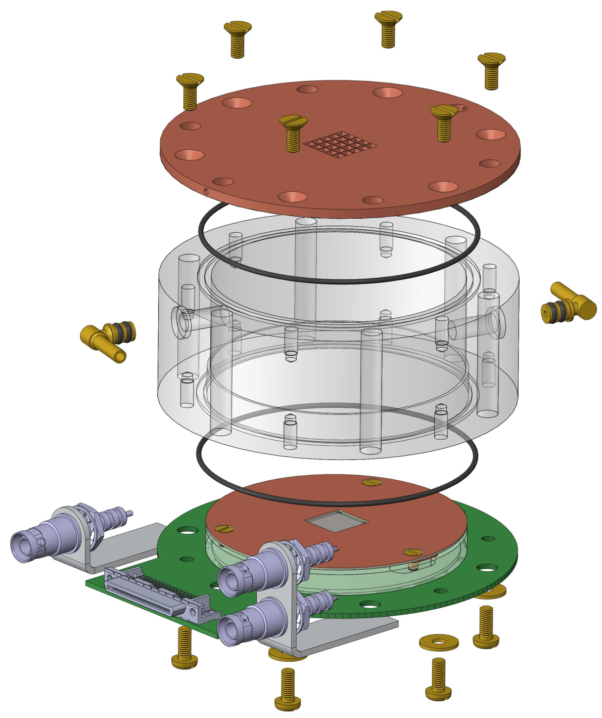
The detector consists of a single GridPix in a \(\SI{78}{mm}\) diameter gas volume and a drift distance of \(\SI{3}{cm}\). The detector has a \(\SI{2}{μm}\) thick Mylar (\(\ce{C10 H8 O4}\)) entrance window for X-rays. This detector serves as the foundation the detector used in the course of this thesis was built on. See fig. 3 for an exploded schematic of the detector. Further, fig. 4 shows the achieved background rate of this detector in the center \(\num{5} \times \SI{5}{mm^2}\) region of the detector. The background rate shows the copper Kα line near \(\SI{8}{keV}\), possibly overlaid with a muon contribution as well as the expected argon Kα lines at \(\SI{3}{keV}\). Below \(\SI{2}{keV}\) the background rises the lower the energy becomes, likely due to background- and signal-like events being less geometrically different at low energies (fewer pixels). The average background rate in the range from \(\SIrange{0}{8}{keV}\) is \(\sim\SI{2.9e-05}{keV^{-1}.cm^{-2}.s^{-1}}\).

7.4.1. Create background rate plot for 2014 data extended
We simply generate the code with our background rate plotting script, as the 2014/15 dataset background rate is stored in our resources of the TPA repository. It also outputs the integrated background rates.
  plotBackgroundRate --show2014 --energyMax 10.0 \
  --title "Background rate in center 5·5 mm² for GridPix 2014/15 CAST data" \
  --useTeX \
  --outpath ~/phd/Figs/ \
  --outfile background_rate_2014_gold.pdf
7.5. Septemboard detector overview
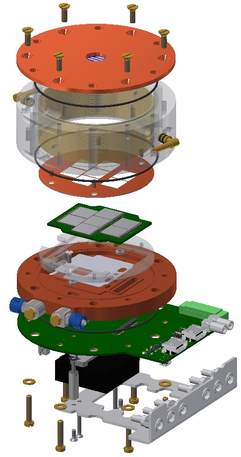
Generally, the detector follows the same design as the old detector shown in sec. 7.4, mainly so that mounting it inside of the lead shielding and to the vacuum pipes at CAST is possible without significant changes. An exploded view of the full detector can be seen in fig. 5.
At the center of the new detector is the 'septemboard', 7 GridPixes replace the single GridPix on the carrier board, sec. 7.10. Analogue signals induced by the amplified charges on the center GridPix are now read out using a flash ADC (FADC), sec. 7.8. The housing with an inner diameter of \(\SI{78}{mm}\) is again made of acrylic glass, same as in the old detector. The detector entrance window is replaced by a \(\SI{300}{nm}\) \ccsini window (sec. 7.9), which also acts as part of the detector cathode. The copper anode slots in right above the septemboard. The carrier board sits on the intermediate board. Below the intermediate board is a bespoke water cooling made of oxygen-free copper to cool the heat emitted by the additional 6 GridPixes, sec. 7.11. On the underside of the intermediate board is a new small silicone photomultiplier (SiPM), sec. 7.7. Finally, a large veto scintillator is installed above the detector setup at CAST, also sec. 7.7.
During developments multiple septemboards were built and tested. The septemboard used in the final detector is septemboard 'H'. The GridPixes of the final board are listed in tab. 5.
| Chip | Number |
|---|---|
| E 6 W69 | 0 |
| K 6 W69 | 1 |
| H 9 W69 | 2 |
| H10 W69 | 3 |
| G10 W69 | 4 |
| D 9 W69 | 5 |
| L 8 W69 | 6 |
7.6. Detector readout system
The detector is operated by a Xilinx Virtex-6 \textbf{F}ield \textbf{P}rogrammable \textbf{G}ate \textbf{A}rray (FPGA) in the form of a Virtex-6 ML605 evaluation board. 3 It is connected to the intermediate board via two \textbf{H}igh-\textbf{D}efinition \textbf{M}ultimedia \textbf{I}nterface (HDMI) cables. The Virtex-6 contains the firmware controlling the Timepix ASICs and correlating the scintillator and FADC signals (see appendix sec. 17.1), the Timepix Operating Firmware (TOF). The high voltage (HV) supply both for the septemboard as well as for the scintillators sit inside a VME crate, which also houses the FADC. A USB connection is used to read out and control the FADC and HV supply via the computer running the data acquisition and control software (see sec. 17.2), the Timepix Operating Software (TOS). A schematic of this setup is shown in fig. 6, which leaves out the SiPM and temperature readout.

7.7. Scintillator vetoes
The first general improvement is the addition of two scintillators for veto purposes. While both have slightly different goals, each is there to help with the removal of muon signals or muon induced events (for example X-ray fluorescence) in the detector. Given that cosmic muons (ref. section 6.2) dominate the background by flux, statistically there is a high chance of muons creating X-ray like signatures in the detector. By tagging muons before they interact near the detector, these can be correlated with events seen on the GridPix and thus possibly be vetoed if precise time information is available.
The first scintillator is a large 'paddle' installed above the detector and beamline, aiming to tag a large fraction of cosmic muons traversing in the area around the detector. It has a Canberra 2007 base and the photomultiplier tube (PMT) is a Bicron Corp. 31.49x15.74M2BC408/2-X (first two numbers: dimensions in inches). The full outer dimensions of the scintillator paddle are closer to \(\SI{42}{cm} \times \SI{82}{cm}\). It is the same scintillator paddle used during the Micromegas data taking behind the LLNL telescope prior and after the data taking campaign with the detector described in this thesis.
For this scintillator, muons which traverse through it and the gaseous detector volume are not the main use case. They can be easily identified by the geometric properties of the induced tracks (their zenith angles are relatively small, resulting in track like signatures as the GridPix readout is orthogonal to the zenith angle). There is a small chance however that a muon can ionize an atom of the detector material, which may emit an X-ray upon recombination. One particular source of background can be attributed to the presence of copper whose Kα lines are at \(\sim\SI{8.04}{\keV}\) as well as fluorescence of the argon gas with its Kα lines at \(\sim\SI{2.95}{keV}\) (see. table 1 in sec. 6.1.4 and sec. 6.1.4).
Fig. 7(a) shows a schematic of a side view of the detector chamber with the scintillator paddle on top. When a muon traverses the scintillator, a counter \(t_{\text{Veto}}\) starts on the FPGA. Two different cases are shown. In the extreme, a muon may traverse close to the cathode or close to the anode / readout plane. This changes the time of the total drift time and therefore the time difference between the trigger time \(t_{\text{Veto}}\) and the readout time, which in the readout is precisely the value of the counter on the FPGA. The drift velocity of \(\sim\SI{2}{cm.μs⁻¹}\) and height of the detector chamber (\(\SI{3}{cm}\)) therefore allow to set an upper limit on the maximum time between a veto paddle trigger and the GridPix readout of about \(\SI{1.5}{μs}\). At a clock speed of \(\SI{40}{MHz}\) this corresponds to \(\SI{60}{clock\;cycles}\), a number we will later try to see in the data (see sec. 12.5.1). As the location at which the muon traverses through the detector is random and homogeneous throughout the detection volume, we expect to see a flat distribution up to the maximum possible time and then a sharp drop (equivalent to muons at the cathode).
The second scintillator is a small silicon photomultiplier (SiPM) installed on the underside of the PCB on which the septemboard is installed. This scintillator was calibrated and set up as part of (Schmitz 2017). We are interested in tagging precisely those muons, which enter the detector orthogonally to the readout plane. This implies zenith angles of almost \(\SI{90}{°}\) such that the elongation in the transverse direction of the muon track is small enough to result in a small eccentricity. From the Bethe equation the mean energy loss of muons in the used gas mixture is about \(\SI{8}{\keV}\) along the \(\SI{3}{\cm}\) of drift volume in the detector (see fig. 11 for the energy loss). This coincides with the copper Kα lines and should lead to another source of background in this energy range. Although the muon background will have a much wider energy distribution than the copper lines, which are dominated by the energy resolution of the detector. In a similar manner to the veto paddle we can make an estimate on the typical time scales associated from the time of the scintillator trigger to the GridPix detection. A muon that traverses orthogonally trough the detector can be taken to leave an instant ionization track and trigger the SiPM at the same time (\(\mathcal{O}(\SI{100}{ps}) \ll \SI{25}{ns}\) for one clock cycle). As such, the relevant time scale is the drift time until enough charge has drifted towards the grid as to pass the activation threshold.
Ionization of a muon is a statistical process, as indicated in fig. 7(b). Depending on the density of the charge cloud for muons orthogonal to readout plane, time to accumulate enough charge to trigger FADC differs. With an average energy deposition of a muon in argon gas of \(\sim\SI{2.67}{keV.cm^{-1}}\), and drift velocity again of \(\SI{2}{cm.μs⁻¹}\) the accumulation time can be estimated. For example assuming an FADC activation threshold of \(\SI{1.5}{keV}\) the necessary charge is accumulated on \(\SI{0.56}{cm}\), which takes about \(\SI{280}{ns} \approx \SI{11}{clock.cycles}\) to accumulate. Different tracks will have deposited different amounts of energy. Therefore, we expect a peak at relatively low clock cycles with a tail up to the same \(\SI{60}{clock.cycles}\) (in case the full \(\SI{3}{cm}\) track needs to be accumulated to activate the FADC).


7.7.1. Discussion of orthogonal muons on the FADC extended
While writing the thesis at some point I had the following thoughs:
[ ]QUESTION: This is VERY IMPORTANT for our interpretation. Given the 'slow' drift velocity of about 2cm/μs, this means orthogonal muons of course take about 1.5μs to traverse the detector. The FADC trigger window is 2560 ns = 2.56 μs. So: Does the FADC even TRIGGER if the charge accumulates that slowly??? UHHHHHH I mean from this we expect to have signals that are extremely long, no? 1.5/2.5 = 0.58 of the whole trigger window! In RISING EDGE Or rather a sort of flat thing, as the charge is removed 'quickly' on those time scales. Very confusing thought…. I mean there is a chance the FADC DID NOT trigger in those events, which could explain why the FADC + SIPM aren't that effective! -> We could study this a bit, if we look into the FADC dataset in which we placed the detector towards the zenith. Question: what does the data look like, in which the FADC DID NOT TRIGGER? If there is significant contribution of spherical events of ~8 keV then DUHHH.
To investigate this we can use plotData from TimepixAnalysis to
make a bunch of plots comparing properties like the energy of clusters
with and without FADC. Both for the raw data as well as for the
results of the likelihood application (i.e. after all cuts).
We will use the entire Run-3 dataset for both cases, because the scintillators were fully working in those.
First the plots of the raw data without FADC:
  plotData \
    --h5file ~/CastData/data/DataRuns2018_Reco.h5 \
    --runType=rtBackground \
    --config ~/CastData/ExternCode/TimepixAnalysis/Plotting/karaPlot/config.toml \
    --ingrid --fadc \
    --cuts '("../fadcReadout", -0.1, 0.5)' \
    --applyAllCuts \
    --chips 3 \
    --region crGold
where we only plot chip 3 in the center 5·5 cm² and apply the cut to
the fadcReadout flag (such that we avoid any floating point
issues). fadcReadout == 0 means no FADC and 1 means FADC.
Let's wrap them all up in one PDF:
    dir=figs/DataRuns2018_Reco_2023-10-03_22-41-58
pdfunite $dir/*.pdf run3_no_fadc_histograms.pdf

Now the same with the FADC. Note for this plot change the rise time
in config.toml to 2500 upper and 500 bins!
  plotData \
    --h5file ~/CastData/data/DataRuns2018_Reco.h5 \
    --runType=rtBackground \
    --config ~/CastData/ExternCode/TimepixAnalysis/Plotting/karaPlot/config.toml \
    --ingrid --fadc \
    --cuts '("../fadcReadout", 0.5, 1.1)' \
    --applyAllCuts \
    --chips 3 \
    --region crGold \
    --quiet
Let's wrap them all up in one PDF:
    dir=figs/DataRuns2018_Reco_2023-10-03_23-45-37
pdfunite $dir/*.pdf run3_with_fadc_histograms.pdf

And now for the result of the data with all cuts applied:
  plotData \
    --h5file ~/org/resources/lhood_lnL_04_07_23/lhood_c18_R3_crAll_sEff_0.8_lnL_scinti_fadc_septem_line_vQ_0.99_default_cluster.h5 \
    --runType=rtBackground \
    --config ~/CastData/ExternCode/TimepixAnalysis/Plotting/karaPlot/config.toml \
    --ingrid --fadc \
    --cuts '("../fadcReadout", -0.1, 0.5)' \
    --applyAllCuts \
    --chips 3 \
    --region crGold
    dir=figs/lhood_c18_R3_crAll_sEff_0.8_lnL_scinti_fadc_septem_line_vQ_0.99_default_cluster_2023-10-03_22-46-10
pdfunite $dir/*.pdf run3_lhood_no_fadc_histograms.pdf

  plotData \
    --h5file ~/org/resources/lhood_lnL_04_07_23/lhood_c18_R3_crAll_sEff_0.8_lnL_scinti_fadc_septem_line_vQ_0.99_default_cluster.h5 \
    --runType=rtBackground \
    --config ~/CastData/ExternCode/TimepixAnalysis/Plotting/karaPlot/config.toml \
    --ingrid --fadc \
    --cuts '("../fadcReadout", 0.5, 1.1)' \
    --applyAllCuts \
    --chips 3 \
    --region crGold
    dir=figs/lhood_c18_R3_crAll_sEff_0.8_lnL_scinti_fadc_septem_line_vQ_0.99_default_cluster_2023-10-03_22-46-44
pdfunite $dir/*.pdf run3_lhood_with_fadc_histograms.pdf

To summarize the results:
-
-> This file shows that there are barely any events near the
\(\SI{8}{keV}\) range for events without an FADC trigger. This already
seems to indicate that orthogonal muons should be triggering the
FADC.
-
-> Shows much higher statistics in the same range. Rise time shows a
very long tail, but no visible peaks at higher values.
-
-> There are literally no events in the \(\SI{8}{keV}\) range after
the likelihood cuts without an FADC trigger!
-
-> There are plenty of events in the \(\SI{8}{keV}\) range after
the likelihood cuts with the FADC. And all their rise times are
between 45 and 70 clock cycles! This means either there are no
orthogonal muons in this dataset or for some reason their rise time
is also exceptionally short, which seems surprising.
At this point we could investigate further and see what the correlation of rise times actually looks like more generally, but well. At least for all data the rise time looks unsuspicious. It's just a long exponential like tail.
7.7.2. Maximum allowed angle before being vetoed extended
The section below explains the reasoning behind why an angle of \(\SI{88}{°}\) was chosen when computing the muon flux at CAST under shallow angles in sec. 6.2.1 and why this is the smallest angle at which a muon is likely going to pass the normal likelihood cut and thus requires the SiPM.
The reason ϑ = 88° was chosen is due to the restriction on the maximum
allowed eccentricity for a cluster to still end up as a possible
cluster in our 8-10 keV hump. See the eccentricity subplot in
fig. 12.

From this we can deduce the eccentricity should be smaller than ε = 1.3. What does this imply for the largest possible angles allowed in our detector? And how does the opening of the "lead pipe window" correspond to this?
Let's compute by modeling a muon track as a cylinder. Reading off the
mean width from the above fig. to w = 5 mm and taking into account
the detector height of 3 cm we can compute the relation between
different angles and corresponding eccentricities.
In addition we will compute the largest possible angle a muon (from the front of the detector of course) can enter, under which it does not see the lead shielding.
    import unchained, ggplotnim, strformat, sequtils
let w = 5.mm #   mean width of a track in 8-10keV hump
let h = 3.cm #   detector height
proc computeLength  (α: UnitLess  ): mm =  ## todo: add degrees?
  ## α: float # Incidence angle
  var w_prime = w / cos(α)       #   projected width taking incidence
                                 #   angle into account
  let L_prime = tan(α) * h       #   projected `  'length'  ` of track
                                 #   from center to center
  let L_full = L_prime + w_prime #   full `  'length'  ` is bottom to top, thus
                                 #   + w_prime
  result = L_full.to(mm)
proc computeEccentricity  (  L_full, w: mm, α: UnitLess  ): UnitLess =
  let w_prime = w / cos(α)
  result = L_full / w_prime

let αs = linspace(  0.0, degToRad(  25.0  ), 1000  )
let εs = αs.mapIt(it.computeLength.computeEccentricity(w, it).float  )
let αsDeg = αs.mapIt(it.radToDeg)
let df = toDf(αsDeg, εs)

#   maximum eccentricity for text annotation
let max_εs = max  (εs)
let max_αs = max  (αsDeg)

#   compute the maximum angle under which `  no  ` lead is seen
let d_open = 28.cm #   assume 28 cm from readout to end of lead shielding
let h_open = 5.cm #   assume open height is 10 cm, so 5 cm from center
let α_limit = arctan(h_open / d_open).radToDeg

#   data for the limit of 8-10 keV eccentricity
let ε_max_hump = 1.3 #   1.2 is more reasonable, but 1.3 is the
                     #   absolute upper limit
echo df.head(  1  )
echo α_limit
echo ε_max_hump
echo max_εs
echo max_αs
ggplot(df, aes(  "αsDeg", "εs"  )  ) +
  geom_line() +
  geom_linerange(aes = aes(x = α_limit, yMin = 1.0, yMax = max_εs),
                 color = color(  1.0, 0.0, 1.0  )  ) +
  geom_linerange(aes = aes(y = ε_max_hump, xMin = 0, xMax = max_αs),
                 color = color(  0.0, 1.0, 1.0  )  ) +
  geom_text(aes = aes(x = α_limit, y = max_εs + 0.1,
                      text = "Maximum angle no lead traversed"  )  ) +
  geom_text(aes = aes(x = 17.5, y = ε_max_hump + 0.1,
                      text = r"Largest $ε$ in $\SIrange{8}{10}{keV}$ hump"  )  ) +
  xlab(r"$α$: Incidence angle [°]"  ) +
  ylab(r"$ε$: Eccentricity"  ) +
  ylim(  1.0, 4.0  ) +
  ggtitle(&"Expected eccentricity for tracks of mean width {w}"  ) +
  ggsave(  "~/phd/Figs/muonStudies/exp_eccentricity_given_incidence_angle.pdf", useTeX = true, standalone = true,
        width = 600, height = 360  )
Resulting in fig. 13.

This leads to an upper bound of ~3° from the horizontal. Hence the (somewhat arbitrary choice) of 88° for the ϑ angle above.
7.8. FADC
As the Timepix is read out in a shutter based fashion and typical shutter lengths for low rate experiments are long compared to the rate of cosmic muons, the scintillators introduced in previous section require an external trigger to close the Timepix shutter early if a signal is measured on the Timepix. This is one the main purposes of the \text{f}lash \textbf{a}nalog to \textbf{d}igital \textbf{c}onverter (FADC) that is part of the detector. This is done by decoupling the induced analogue signals from the grid of the center GridPix.
The specific FADC used for the detector is a Caen V1792a. It runs at an internal \(\SI{50}{MHz}\) or \(\SI{100}{MHz}\) clock and utilizes virtual frequency multiplication to achieve sampling rates of \(\SI{1}{GHz}\) or \(\SI{2}{GHz}\), respectively. It has 4 channels, each with a cyclic register of \(\num{2560}\) channels. At an operating clock frequency of \(\SI{1}{GHz}\) that means each channel covers the last \(\sim\SI{2.5}{\micro\second}\) at any time. (CAEN 2010)
The raw signal decoupled from the grid is first fed into an Ortec 142 B pre-amplifier and then feeds into an Ortec 474 shaping amplifier, which integrates and shapes the signal as well as amplifies it. For a detailed introduction to this FADC system, see the thesis of A. Deisting (Deisting 2014) and (Schmidt 2016) for further work integrating it into this detector. In addition see the FADC manual (CAEN 2010) 4 for a deep explanation of the working principle of this FADC.
The analogue signal of the center grid is decoupled via a small \(C_{\text{dec}} = \SI{10}{nF}\) capacitor in parallel to the high voltage line. For a schematic of the circuit see fig. 14. When a primary electron traverses through a hole in the grid and is amplified, the back flowing ions induce a small voltage spike on top of the constant high voltage applied to the grid. The parallel capacitor filters out the constant high voltage and only transmits the time varying induced signals. Such signals – the envelope of possibly many primary electrons – are measured by the FADC.

This signal can be used for three distinct things:
- it may be used as a trigger to close the shutter of the ongoing event. Ideally, we want to only measure a single physical event within one shutter window. A long shutter time can statistically result in multiple events happening, which the FADC trigger helps to alleviate. This allows us to reduce the number of events with multiple physical events and acts as a trigger for the scintillators. This in turn means possible muon induced X-ray fluorescence can be vetoed.
- By nature of the signal production and drift properties of the primary electrons before they reach the grid, the signal shape can theoretically be used to determine a rough longitudinal shape of the event. The length of the FADC event should be proportional to the size of the primary electron cloud distribution along the 'vertical' detector axis. This potentially allows to differentiate between a muon traversing orthogonally through the readout plane and an X-ray due to their longitudinal shape difference, see sec. 12.5.2.
- Finally, it provides an independent measure of the collected charge on the center chip. This will prove useful in understanding the detector behavior over time later in sec. 11.2.2.
The working principle of how the FADC and the scintillators can be used together to remove certain types of background, by correlating events in the scintillators, the FADC and the GridPix, is shown in fig. 15.

7.8.1. Update schematic extended
Need to type out μs because we don't use unicode-math by default in LaTeXDSL.
    import latexdsl
let body = r"If $Δt \lesssim \mathcal{O}(\SI{2}{\micro\second})$ events considered correlated, flag them."
compile(  "/tmp/text_fadc_scintillator.tex", body)
7.9. SiN window
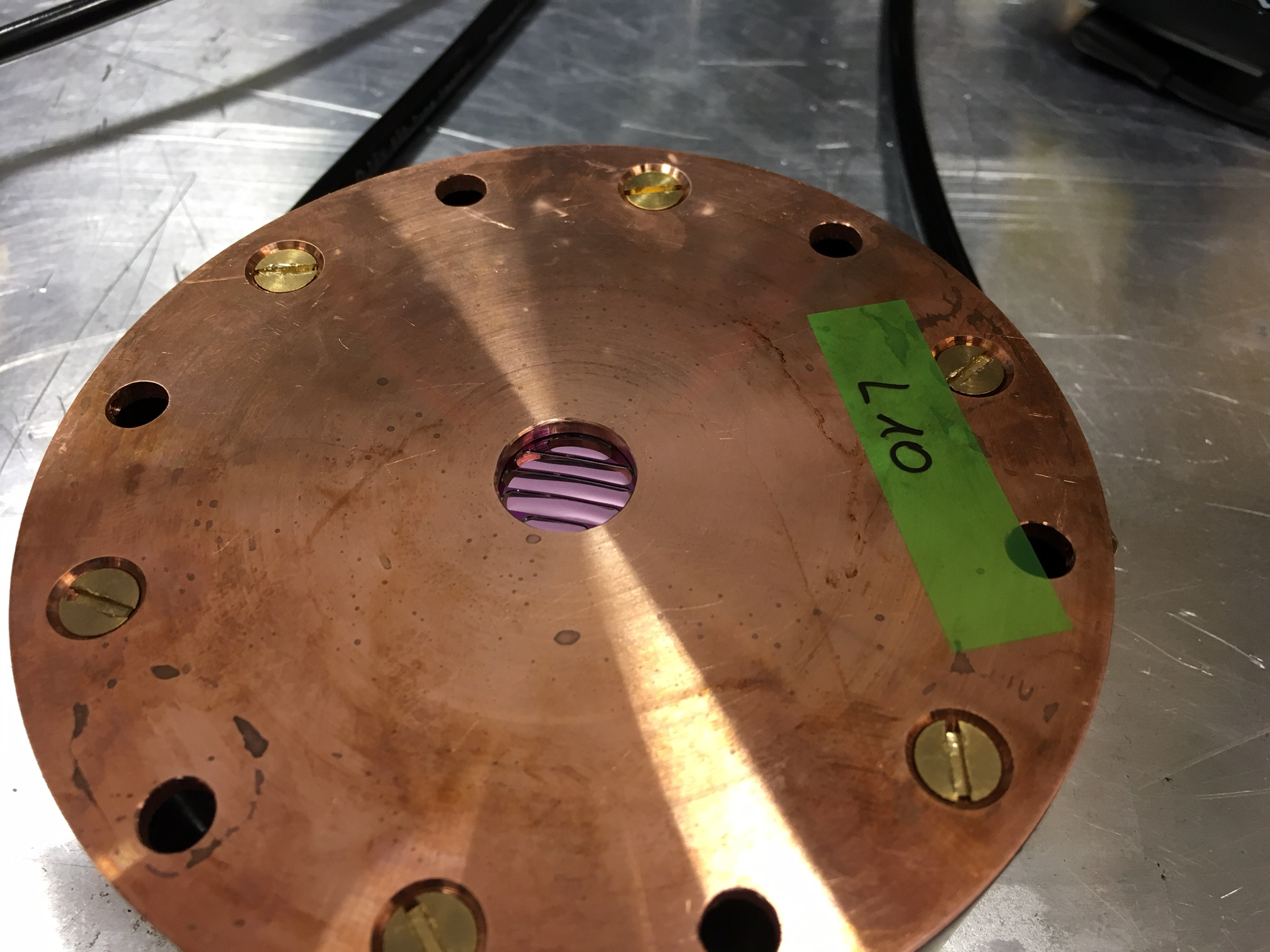
Next up, a major limitation of the previous detector was its limited combined efficiency below \(\SI{2}{keV}\), due to its \(\SI{2}{μm}\) Mylar window. Therefore, the next improvement for the new detector is an ultra-thin silicon nitride \(\ce{Si_3 N_4}\) window of \(\SI{300}{nm}\) thickness and \(\SI{14}{mm}\) diameter, developed by Norcada 5. A strongback support structure consisting of 4 lines of \(\SI{200}{μm}\) thick and \(\SI{500}{μm}\) wide \(\ce{Si_3 N_4}\), helps to support a pressure difference of up to \(\SI{1.5}{bar}\). On the outer side a \(\SI{20}{nm}\) thin layer of aluminum is coated to allow the window to be part of the detector cathode. The strongback occludes about \(\SI{17}{\%}\) of the full window area. In reality it is slightly more, as the strongbacks become somewhat wider towards the edges. In the centermost region they are straight and in the center \(\num{5} \times \SI{5}{mm²}\) area, they occlude \(\SI{22.2}{\%}\).
Fig. 16(a) shows the idealized strongback structure without a widening towards the edges of the window. Fig. 16(b) shows an image of one such window under testing conditions in the laboratory, as it withstands a pressure difference of \(\SI{1.5}{bar}\).

As the main purpose is the increase of transmission at low energies, fig. 17 shows the transmission of the mylar window of the old detector and the new \(\ce{Si_3 N_4}\) window in the energy range below \(\SI{3}{keV}\). The \(\ce{Si_3 N_4}\) window shows a significant increase in transmission below \(\SI{2}{keV}\), which is very important for the sensitivity in solar axion-electron and chameleon searches, which both peak near \(\SI{1}{keV}\) in their solar flux. The window alone significantly increases the signal to noise ratio of these physics searches.

7.9.1. Calculation of strongback window structure plot extended
    ## Super dumb MC sampling over the entrance window using the Johanna's code from `  raytracer2018.nim  `
## to check the coverage of the strongback of the 2018 window
##
## Of course one could just color areas based on the analytical description of where the
## strongbacks are, but this is more interesting and looks fun. The good thing is it also
## allows us to easily compute the fraction of pixels within and outside the strongbacks.
import ggplotnim, random, chroma
proc colorMe  (y: float  ): bool =
  const
    stripDistWindow = 2.3  #  mm
    stripWidthWindow = 0.5 #  mm
  if abs  (y) > stripDistWindow / 2.0 and
     abs  (y) < stripDistWindow / 2.0 + stripWidthWindow or
     abs  (y) > 1.5 * stripDistWindow + stripWidthWindow and
     abs  (y) < 1.5 * stripDistWindow + 2.0 * stripWidthWindow:
    result = true
  else:
    result = false

proc sample  () =
  randomize(  423  )
  const nmc = 5_000_000
  let black = color(  0.0, 0.0, 0.0  )
  var dataX = newSeqOfCap[  float  ](nmc)
  var dataY = newSeqOfCap[  float  ](nmc)
  var strongback = newSeqOfCap[  bool  ](nmc)
  for idx in 0 ..< nmc:
    let x = rand(-7.0 .. 7.0  )
    let y = rand(-7.0 .. 7.0  )
    if x*x + y*y < 7.0 * 7.0:
      dataX.add x
      dataY.add y
      strongback.add colorMe(y)
  let df = toDf(dataX, dataY, strongback)
  echo "A fraction of ", df.filter(f{`strongback` == true  }  ).len / df.len, " is occluded by the strongback"
  let dfGold = df.filter(f{  abs  (idx(`dataX`, float  )  ) <= 2.25 and
                           abs  (idx(`dataY`, float  )  ) <= 2.25  }  )
  echo "Gold region: A fraction of ", dfGold.filter(f{`strongback` == true  }  ).len / dfGold.len, " is occluded by the strongback"
  ggplot(df, aes(  "dataX", "dataY", fill = "strongback"  )  ) +
    geom_point(size = 1.0  ) +
    #   draw the gold region as a black rectangle
    geom_linerange(aes = aes(y = 0, x = 2.25, yMin = -2.25, yMax = 2.25  ), color = "black"  ) +
    geom_linerange(aes = aes(y = 0, x = -2.25, yMin = -2.25, yMax = 2.25  ), color = "black"  ) +
    geom_linerange(aes = aes(x = 0, y = 2.25, xMin = -2.25, xMax = 2.25  ), color = "black"  ) +
    geom_linerange(aes = aes(x = 0, y = -2.25, xMin = -2.25, xMax = 2.25  ), color = "black"  ) +
    xlab(  "x [mm]"  ) + ylab(  "y [mm]"  ) +
    ggtitle(  "Idealized layout, strongback in purple"  ) +
    themeLatex(fWidth = 0.5, width = 640, height = 480, baseTheme = sideBySide) +
    ggsave(  "/home/basti/phd/Figs/SiN_window_occlusion.pdf", useTeX = true, standalone = true, dataAsBitmap = true  )  #  width = 1150, height = 1000)
sample()
7.10. Septemboard - 6 GridPixes around a center one
The main motivation for extending the readout area from a single chip to a 7 chip readout is to reduce background towards the outer sides of the chip, in particular in the corners. Against common intuition however, it also plays a role for events which have cluster centers near the center of the readout. The latter is, because diffusion can produce quite large clusters even at low energies. In particular in lower energy events, tracks may have gaps in them large enough to avoid being detected as a single cluster for standard radii in cluster searching algorithms. This is particularly of interest as different searches produce an 'image' at different positions and sizes on the detector. While the center chip is large enough to fully cover the image for essentially all models, it may not be in the regions of lowest background. Hence, improvements to larger areas are needed.
The septemboard is implemented in such a way to optimize the loss of active area due to bonding requirements and general manufacturing realities. As the Timepix ASIC is a \(\SI{16.1}{mm}\) by \(\SI{14.1}{mm}\) large chip (the bonding area adding \(\SI{2}{mm}\) on one side), the upper two rows are installed such that they are inverted to another. The bonding area is above the upper row and below the center row. The bottom row again has its bonding area below. This way the top two rows are as close together as realistically possible, with a decent gap on the order of \(\SI{2}{mm}\) between the middle and bottom row. Any gap is potentially problematic as it implies loss of signal in that area, complicating the possible reconstruction methods. The layout can be seen in fig. 20 in the next section.
All 7 GridPix are connected in a daisy-chained way. This means that in particular for data readout, all chips are read out in serial order. The dead time for readouts therefore is approximately 7 times the readout time of a single Timepix. A single Timepix has a readout time of \(\sim\SI{25}{ms}\) at a clock frequency of \(\SI{40}{MHz}\) (the frequency used for this detector). This leads to an expected readout time of the full septemboard of \(\SI{175}{ms}\). 6 Such a long readout time leads to a strong restriction of the possible applications for such a detector. Fortunately, for the use cases in a very low rate experiment such as CAST, long shutter times are possible, mitigating the effect on the fractional dead time to a large extent.
Fig. 18 shows a heatmap of all cluster centers during roughly \(\SI{2000}{h}\) of background data after passing these clusters through a likelihood based cut method aiming to filter out non X-ray like clusters (details of this follow later in sec. 12.1). It is clearly visible that the further a cluster center is towards the chip edges, and especially the corners, the more likely it is to be considered an X-ray like cluster. This has an easy geometric explanation. Consider a perfect track traversing over the whole chip. In this case it is very eccentric. Move the same track such that its center is in one of the corners and rotate it by \(\SI{45}{°}\) and suddenly the majority of the track won't be detected on the chip anymore. Instead something roughly circular remains visible, 'fooling' the likelihood method. For a schematic illustrating this, see fig. 19.
The septemboard therefore is expected to significantly reduce the background over the whole center chip, with the biggest effect in the regions with the most amount of background.


7.10.1. GridPix veto ring illustration extended
The event used in the illustration is event 23707 of run 242.
The full event display:

and the SVG of the illustration:

7.10.2. Compute the cluster backgrounds extended
To compute these cluster backgrounds, we need the following ingredients:
- the fully reconstructed data files
DataRuns201*_Reco.h5 - the prepared CDL data from the 2019 dataset
calibration-cdl_2019.h5and the X-ray reference datasets that define the X-ray like properties. - apply the likelihood method to all background events in one of the files (gives enough statistics) to get a resulting file containing only passed clusters over the whole chip.
With the resulting file we can then use ./../CastData/ExternCode/TimepixAnalysis/Plotting/plotBackgroundClusters/plotBackgroundClusters.nim to plot these cluster centers.
Assuming the reconstructed data files are found in … and the CDL data files in …, let's generate the data after likelihood method: (this takes ~2 minutes or so, so better run it in a terminal instead of via C-c C-c)
  likelihood \
    -f ~/CastData/data/DataRuns2017_Reco.h5 \
    --h5out /tmp/lhood_2017_full_chip.h5 \
    --cdlYear=2018 \
    --region=crAll \
    --cdlFile=/home/basti/CastData/data/CDL_2019/calibration-cdl-2018.h5 \
    --lnL
[ ]WHY DOES THIS produce background suppression numbers below 1 towards the corners?
Compile the plotting tool if not done:
nim c -d:danger --threads:on plotBackgroundClusters.nim
Now we can create the plot. Note that we use fWidth = 0.8 so that
(as of right now ) the heatmap fits on one page
with the septem veto illustration.
  plotBackgroundClusters \
    -f ~/org/resources/lhood_lnL_17_11_23_septem_fixed/lhood_c18_R2_crAll_sEff_0.8_lnL.h5 \
    --title "2000 h background data, lnL cut applied" \
    --outpath ~/phd/Figs/backgroundClusters/ \
    --energyMin 0.2 \
    --energyMax 12.0 \
    --zMax 15.0 \
    --singlePlot \
    --fWidth 0.8 \
    --useTikZ
7.11. Water cooling and temperature readout for the septemboard
During development of the septemboard one particular set of problems manifested. While testing a prototype board with 5 active GridPix in a gaseous detector, the readout was plagued by excessive noise problems. The detector exhibited a large number of frames with more than \(\num{4096}\) active pixels (the limit for a zero suppressed readout) and common pixel values of \(\num{11810}\) indicating overrun ToT counters. On an occupancy (sum of all active pixels) of the individual chips, it is quite visible the data is clearly not due to cosmic background. Fig. 20 shows such an occupancy with the color scale topping out at the \(80^{\text{th}}\) percentile of the counts for each chip individually. The chip in the bottom left shows a large number of sparks (overlapping half ellipses pointing downwards) at the top end. Especially the center chip in the top row shows highly structured activity, which is in contrast to the expectation of a homogeneous occupancy for a normal background run. In addition, on all chips some level of general noise on certain pixels is visible (some being clearly more active than others resulting in a scatter of 'points').

The intermediate board and carrier board used during these tests were
the first boards equipped with two PT1000 temperature sensors. One on
the bottom side of the carrier board and another on the intermediate
board. Each is read out using a MAX31685 micro controllers. Both of
which are communicated with via a MCP2210 USB-to-SPI micro
controllers over a single USB port on the intermediate board. The
single MCP2210 communicates with both temperature sensors via the
Serial Peripheral Interface (SPI) (see
sec. 17.2.4 for more information about the
temperature logging and readout). In the run shown in
fig. 20 the temperature sensors
were not functional yet, as the readout software was not written. The
required logic was added to the Timepix Operating Software (TOS), the
readout software of the detector, motivated by this noise activity to
monitor the temperature before and during a data taking period. The
temperature on the carrier board indicated temperatures of
\(\sim\SI{75}{\celsius}\) in background runs similar to the one of
fig. 20. One way to get a measure
for the noise-like activity seen on the detector is to look at the
rate of active pixels over time. With values well above numbers
expected due to background, excess temperature seemed a possible cause
for the issues. As no proper cooling mechanism was available, a
regular desk fan was placed pointing at the detector when it was run
without any kind of shielding. This saw the temperature under the
carrier board drop from \(\SI{76}{\celsius}\) down to
\(\SI{68}{\celsius}\). As a result the majority of noise disappeared as
can be seen in fig. 21(b)
with the temperature curve during the full run in
fig. 21(a). 7 , 8
The features visible in the occupancy plots are thus likely multiple different artifacts due to too high temperatures. A mixture of real sparks (bottom left chip in fig. 20) and possible instabilities that possibly affect voltages for the pixels (and thus change the thresholds of each pixel). As the temperature is measured on the bottom side of the carrier board, temperatures in the amplification region are likely higher.


Following this a bespoke water cooling was designed by T. Schiffer, made from oxygen-free copper with \(\SI{3}{mm}\) channels for water to circulate through the copper body. (Schiffer 2024) The body has the same diameter as the intermediate board and is installed right below. The water circulation is handled by an off-the-shelf pump and radiator from Alphacool 9 intended for water cooling setups for desktop computers. The pump manages a water flow rate of about \(\SI{0.3}{\liter\per\minute}\) through the \(\SI{3}{mm}\) channels in the copper. In common operation the temperatures on the carrier board are between \(\SIrange{45}{50}{\celsius}\) and noise free operation is possible.
7.11.1. Sparking behavior extended
See the mails containing "Septem F" (among other things) for the information about sparking behavior. From that we can also deduce the run numbers of the noisy runs (run 241 is one of them); just keep in mind that the run numbers are overlapping with some CAST run numbers, as for CAST we started again at 0.
Specific run path of noisy run used in occupancy plot above:
Run_241_170216-13-49
So run from February 2017.
Let's plot the temperature during the sparking run in which we installed the fan.
This is essentially a reproducible version of the following plot:

    import ggplotnim, times

#   Laptop:
#  const path = "/mnt/1TB/CAST/2017/development/Run_268_170418-05-43/temp_log.txt"
#   Desktop:
const path = "~/CastData/data/2017/development/Run_268_170418-05-43/temp_log.txt"

proc p  (x: string  ): DateTime =
  result = x.parse(  "YYYY-MM-dd'.'HH:mm:ss", local()  )
let df = readCsv(path, sep = '\t', skipLines = 2, colNames = @[  "IMB", "Septem", "DateTime"  ]  )
  .filter(f{  string -> bool: p(`DateTime`) < initDateTime(  19, mApr, 2017, 0, 0, 0, 0, local()  )  }  )
  .gather(@[  "IMB", "Septem"  ], "Type", "Temperature"  )
  .mutate(f{  "Timestamp" ~ p(`DateTime`).toTime().toUnix()  }  )

## XXX: fix plotting of string columns as date scales, due to discrete / continuous mismatch and lacking
## `  dataScale  ` field
ggplot(df, aes(  "Timestamp", "Temperature", color = "Type"  )  ) +
  geom_line() +
  #   scale_x_continuous() +
  ggtitle(  "Temperature on 2017/04/18 with fan"  ) +
  xlab(  "Time of day", margin = 3.25, rotate = -45.0, alignTo = "right"  ) + ylab(  "Temperature [°C]"  ) +
  margin(bottom = 4.0, right = 4.0  ) +
  scale_x_date(isTimestamp = true,
               formatString = "HH:mm:ss",
               dateSpacing = initDuration(hours = 2  ),
               dateAlgo = dtaAddDuration,
               timeZone = local()  ) +
  themeLatex(fWidth = 0.5, width = 600, height = 420, baseTheme = sideBySide) +
  ggsave(  "/home/basti/phd/Figs/detector/sparking/temperature_sparking_run_268.pdf",
        width = 600, height = 360, useTeX = true, standalone = true  )
df.writeCsv(  "/home/basti/phd/resources/temperature_sparking_run_268.csv"  )
Next up we need to compute the mean hit rate of the four most active chips and plot it against time.
How will we go about doing that? Read and reconstruct the run, then manually extract hits per time, bin by time and that's it?
    #   cd /mnt/1TB/CAST/2017/development/
cd ~/CastData/data/2017/development/
raw_data_manipulation -p Run_268_170418-05-43 --runType background --out raw_268_sparking.h5
reconstruction -i raw_268_sparking.h5 --out reco_268_sparking.h5
With the resulting file, we can now generate the plot of the hits over time.
This is a reproducible version of the following plot:

    import std / [options, sequtils, times]
import ggplotnim, nimhdf5, unchained
defUnit(Second⁻¹)
import ingrid / tos_helpers
#   Laptop
#   const path = "/mnt/1TB/CAST/2017/development/reco_268_sparking.h5"
#   Desktop
const path = "~/CastData/data/2017/development/reco_268_sparking.h5"
let h5f = H5open  (path, "r"  )

var df = newDataFrame()
var dfR = newDataFrame()
for chip in 0 ..< 5:
  let dsets = @[  "hits"  ]
  let dfC = h5f.readRunDsets(
    268,
    chipDsets = some(  (chip: chip, dsets: dsets)  ),
    commonDsets = @[  "timestamp"  ]
  )
    .mutate(f{  "chip" <- chip}  )
    .arrange(  "timestamp"  )
  df.add dfC

  #   and directly compute the hit frequency
  let hits = dfC[  "hits", int  ]
  let time = dfC[  "timestamp", int  ]
  let ts = time.map_inline(  (x - time[  0  ]  ).s)
  const Interval = 30.min
  var i = 0
  var rate = newSeq  [Second⁻¹]()
  var rateTime = newSeq  [  float  ]()
  while i < time.len:
    var h = 0
    var Δt = 0.s
    let t0 = time[i]
    echo "Starting at t0 = ", t0
    while Δt < Interval and i < time.len:
      h += hits[i]
      if i > 0:
        Δt += ts[i] - ts[i-1  ]
      inc i
    rate.add (h.float / Δt  )
    echo "To ", time[i-1  ]
    rateTime.add  (  (time[i-1  ] + t0) / 2.0  )
    h = 0
  dfR.add toDf(  {  "rate" : rate.mapIt(it.float  ), rateTime, "chip" : chip}  )
echo df
echo dfR

dfR = dfR.filter(f{  int -> bool: fromUnix(`rateTime`).inZone(local()  ) < initDateTime(  19, mApr, 2017, 0, 0, 0, 0, local()  )  }  )
ggplot(dfR, aes(  "rateTime", "rate", color = factor(  "chip"  )  )  ) +
  geom_point() +
  scale_y_log10() +
  scale_x_date(isTimestamp = true,
               formatString = "HH:mm:ss",
               dateSpacing = initDuration(hours = 2  ),
               dateAlgo = dtaAddDuration,
               timeZone = local()  ) +
  themeLatex(fWidth = 0.5, width = 600, height = 420, baseTheme = sideBySide) +
  margin(bottom = 4.0, right = 4.0  ) +
  xlab(  "Time of day", margin = 3.25, rotate = -45.0, alignTo = "right"  ) +
  ylab(r"Rate [$\si{pixel.s^{-1}}$]"  ) +
  ggsave(  "/home/basti/phd/Figs/detector/sparking/mean_hit_rate_sparking_run_268.pdf",
        width = 600, height = 360, useTex = true, standalone = true  )

dfR.writeCsv(  "/home/basti/phd/resources/mean_hit_rate_sparking_run_268.csv", precision = 10  )
Finally, combine both and plot together:
    import std / times
import ggplotnim
const path = "/home/basti/phd/resources/"
let df = readCsv(path & "temperature_sparking_run_268.csv"  )
let dfR = readCsv(path & "mean_hit_rate_sparking_run_268.csv"  )
  .group_by(  "chip"  )
  .mutate(f{  "rateNorm" ~ `rate` / max  (`rate`) * 80.0  }  )
  .rename(f{  "Timestamp" <- "rateTime"  }  )

let sa = secAxis(name = "Hit rate [a.u.]",
                 trans = f{  1.0 / 80.0  }  )
                 #  invTransFn = f{`  rateNorm  ` * 80.0})

ggplot(df, aes(  "Timestamp", "Temperature", color = "Type"  )  ) +
  geom_line() +
  geom_point(data = dfR, aes = aes(  "Timestamp", "rateNorm", color = factor(  "chip"  )  )  ) +
  #   ggtitle("Temperature during run on 2017/04/18 in which fan was placed next to detector") +
  xlab(  "Time of day"  ) + ylab(  "Temperature [°C]"  ) +
  margin(top = 2.0  ) +
  scale_y_continuous(secAxis = sa) +
  scale_x_date(isTimestamp = true,
               formatString = "HH:mm:ss",
               dateSpacing = initDuration(hours = 2  ),
               dateAlgo = dtaAddDuration,
               timeZone = local()  ) +
  legendPosition(  0.835, 0.1  ) +
  yMargin(  0.05  ) +
  ggsave(  "/home/basti/phd/Figs/detector/sparking/temperature_and_sparking_run_268.pdf"  )
And finally, let's also recreate the occupancy plot
 of run 241 during
development to showcase the sparking behavior.
of run 241 during
development to showcase the sparking behavior.
In order to do that, we first need to reconstruct the run containing the data:
    cd /mnt/1TB/CAST/2017/development/
raw_data_manipulation -p Run_241_170216-13-49 --runType background --out raw_241_sparking.h5
reconstruction raw_241_sparking.h5 --out reco_241_sparking.h5
With the reconstructed data file at hand, we can first of all generate a large number of plots for each chip:
  plotData --h5file reco_241_sparking.h5 \
         --runType rtBackground \
         --config ~/CastData/ExternCode/TimepixAnalysis/Plotting/karaPlot/config.toml \
         --ingrid --occupancy
which can be adjusted according to the user's preference of course.
(For this plot in particular it's really important not use the ToT
cutting feature in raw_data_manipulation via the rmToTLow and
rmToTHigh in the config.toml file)
With the file in place, let's now create the plot of the occupancies for each chip, embedded in the layout of the septemboard (at least for the 5 chips that were on this septemboard F).
[ ]REPLACE BELOW PLACEMENT BYgeometry.nimIMPLEMENTATION
    import std / os except FileInfo
import std / strutils
import ingrid / [tos_helpers, ingrid_types]
import nimhdf5, ggplotnim, ginger

## The Septemboard layout code is a port of the code used in the python based event
## display for TOS.

const
  Width = 14.1
  Height = 14.1
  BondHeight = 2.0
  FullHeight = Height + BondHeight
  NumChips = 7

  #   If this is set to `  true  ` the final plot will only contain the actual raster image. No legend or axes
  OnlyRaster = true

  Run = 241

type
  SeptemRow = object
    left: float
    right: float
    wspace: float
    top: float
    bottom: float

proc initSeptemRow  (nChips: int, x_size, y_size, x_dist, x_offset, y_t_offset, y_b_offset, dist_to_row_below: float  ): SeptemRow =
  #   this class implements a single row of chips of the septem board
  #   nChips: number of chips in row
  #   x_dist: distance in x direction between each chip
  #   x_offset: offset of left edge of first chip in row from
  #             left side of center row
  #   calculate width and height of row, based on chips and dist
  let width = nChips.float * Width + (nChips - 1  ).float * x_dist
  let height_active = Height
  let height_full = FullHeight + dist_to_row_below
  #   using calc gridspec one calculates the coordinates of the row on
  #   the figure in relative canvas coordinates
  #   include padding by adding or subtracting from left, right, top, bottom
  result.left      = x_offset / x_size
  result.right     = result.left + width / x_size
  result.wspace    = x_dist / x_size
  result.top       = 1.0 - y_t_offset / y_size
  result.bottom    = result.top - height_active / y_size

proc initSeptemBoard  (padding, fig_x_size, fig_y_size, scaling_factor: float  ): seq  [  SeptemRow  ] =
  #   implements the septem board, being built from 3 septem rows

  proc initRows  (y_size, scaled_x_size, scaled_y_size, y_row1_row2, y_row2_row3, row2_x_dist: float  ): seq  [  SeptemRow  ] =
    #   this function creates the row objects for the septem class
    #   calculation of row 1 top and bottom (in abs. coords.):
    let
      #   (top need to add padding to top of row 1)
      row1_y_top    = y_size - BondHeight - Height
      #   bottom in abs. coords.
      row1_y_bottom = 2 * FullHeight + y_row1_row2 + y_row2_row3 - Height
      #   offset of left side from septem in abs. coords.
      row1_x_offset = 6.95
    #   now create the first row with all absolute coordinates
    result.add initSeptemRow(  2, scaled_x_size, scaled_y_size, 0.85, row1_x_offset, row1_y_top, row1_y_bottom, y_row1_row2)
    #   calculation of row 2 top and bottom (top & bottom of row2 not affected by padding):
    let
      row2_y_top    = y_size - FullHeight - y_row1_row2 - Height
      row2_y_bottom = FullHeight + y_row2_row3 + BondHeight - Height
      #   no offset for row2, defines our left most position in abs. coords.
      row2_x_offset = 0.0 #  padding * x_size
    result.add initSeptemRow(  3, scaled_x_size, scaled_y_size, row2_x_dist, row2_x_offset, row2_y_top, row2_y_bottom, y_row2_row3)
    #   calculation of row 3 top and bottom (add padding to bottom):
    let
      row3_y_top    = y_size - 2 * FullHeight - y_row1_row2 - y_row2_row3 - Height
      row3_y_bottom = BondHeight - Height
      row3_x_offset = 7.22
    result.add initSeptemRow(  2, scaled_x_size, scaled_y_size, 0.35, row3_x_offset, row3_y_top, row3_y_bottom, 0  )

  #   include a padding all around the septem event display of 'padding'
  #   use size of figure to scale septem accordingly to have it always properly
  #   scaled for the given figure
  #   take the inverse of the scaling factor (want 1/2 as input to scale to half size)
  let scaling_factor = 1.0 / scaling_factor
  #   first calculate the ratio of the figure
  let fig_ratio = float  (fig_x_size) / float  (fig_y_size)
  #   distances between different rows in absolute coordinates
  let
    y_row1_row2 = 0.38
    y_row2_row3 = 3.1
    #   size in y direction of whole septem board in absolute coordinates
    y_size      = 3 * FullHeight + y_row1_row2 + y_row2_row3
    #   already define row2_x_dist here (in absolute coordinates) to calculate x_size
    row2_x_dist = 0.35
    #   3 chips * width + 2 * distance between chips (in absolute coordinates)
    x_size      = 3 * Width + (  3 - 1  ) * row2_x_dist
  #   calculate the ratio of the septem board
  var ratio = float  (x_size) / float  (y_size)
  #   now calculate the needed ratio to get the correct scaling of the septem on any
  #   figure scale. fig_ratio / own ratio
  ratio = fig_ratio / ratio
  let
    #   scaled x and y sizes
    scaled_x_size = x_size * ratio * scaling_factor
    scaled_y_size = y_size * scaling_factor
  #   and now create the row objects
  result = initRows(y_size, scaled_x_size, scaled_y_size, y_row1_row2, y_row2_row3, row2_x_dist)

proc readVlen  (h5f: H5File,
              fileInfo: FileInfo,
              runNumber: int,
              dsetName: string,
              chipNumber = 0,
              dtype: typedesc = float  ): seq  [  seq  [dtype]  ] =
  ## reads variable length data `  dsetName  ` and returns it
  ## In contrast to `  read  ` this proc does *not* convert the data.
  let vlenDtype = special_type(dtype)
  let dset = h5f[  (fileInfo.dataPath(runNumber, chipNumber).string / dsetName).dset_str]
  result = dset[vlenDType, dtype]

proc calcOccupancy  [  T  ](x, y: seq  [  seq  [  T  ]  ], z: seq  [  seq  [  uint16  ]  ] = @[]  ): Tensor  [  float  ] =
  ## calculates the occupancy of the given x and y datasets
  ## Either for a `  seq[seq[T: SomeInteger]]  ` in which case we're calculating
  ## the occupancy of a raw clusters or `  seq[T: SomeFloat]  ` in which case
  ## we're dealing with center positions of clusters
  result = newTensor[  float  ](  [  NPix, NPix  ]  )
  #   iterate over events
  for i in 0 .. x.high:
    let
      xEv = x[i]
      yEv = y[i]
    var zEv: seq  [  uint16  ]
    if z.len > 0:
      zEv = z[i]
    ## continue if full event.
    ## TODO: replace by solution that also works for clusters!!
    #  if xEv.len >= 4095: continue
    for j in 0 .. xEv.high:
      if zEv.len > 0:
        result  [xEv[j].int, yEv[j].int  ] += zEv[j].float
      else:
        result  [xEv[j].int, yEv[j].int  ] += 1.0

proc occForChip  (h5f: H5File, chip: int, fileInfo: FileInfo  ): (  Tensor  [  int  ], Tensor  [  int  ], Tensor  [  float  ]  ) =
  const NPix = 256
  let
    xD = h5f.readVlen(fileInfo, Run, "x", chip, dtype = uint8  )
    yD = h5f.readVlen(fileInfo, Run, "y", chip, dtype = uint8  )
    zD = h5f.readVlen(fileInfo, Run, "ToT", chip, dtype = uint16  )
  let occ = calcOccupancy(xD, yD) #   , zD)
  var
    x = newTensorUninit[  int  ](  NPix * NPix  )
    y = newTensorUninit[  int  ](  NPix * NPix  )
    z = newTensorUninit[  float  ](  NPix * NPix  )
  var i = 0
  for idx, val in occ:
    x[i] = idx[  0  ]
    y[i] = idx[  1  ]
    z[i] = val
    inc i
  result = (x, y, z)

proc handleOccupancy  (h5f: H5File,
                     chip: int,
                     fileInfo: FileInfo,
                     quant: float = 0.0  ): PlotView =
  #   get x and y datasets, stack and get occupancies
  let (x, y, z) = h5f.occForChip(chip, fileInfo)
  let df = toDf(x, y, z)
  var quant = quant
  if quant == 0.0:
    quant = percentile(z, 80  )
  result = ggcreate(
    block:
      var plt =
        ggplot(df, aes(  "x", "y", fill = "z"  ), backend = bkCairo) +
          geom_raster() +
          scale_fill_continuous(scale = (  low: 0.0, high: quant)  ) + #  high: 1600.0)) +
          xlim(  0, NPix  ) + ylim(  0, NPix  )
      if OnlyRaster:
        plt = plt + theme_void() + hideLegend()
      plt
  )
  #  ggplot(df, aes("x", "y", fill = "z"), backend = bkCairo) +
  #      geom_raster() +
  #      scale_fill_continuous(scale = (low: 0.0, high: 1600.0)) +
  #      xlim(0, NPix) + ylim(0, NPix) +
  #      ggsave("/t/test_occ_0_.pdf")

proc drawBounds  (v: Viewport  ) =
  v.drawBoundary(writeName = true  )
  for ch in mitems  (v.children):
    ch.drawBounds()

proc calcQuantileChip3  (h5f: H5File, fileInfo: FileInfo  ): float =
  let (x, y, z) = h5f.occForChip(  3, fileInfo)
  result = percentile(z, 80  )

proc addRow  (view: Viewport, h5f: H5File, septem: seq  [  SeptemRow  ], fileInfo: FileInfo, i, num, chipStart: int, showEmpty = false  ) =
  let width = septem[i].right - septem[i].left
  let height = septem[i].top - septem[i].bottom

  var row = view.addViewport(left = septem[i].left, bottom = septem[i].bottom,
                             width = width, height = height)
  row.layout(num, 1  ) #  , margin = quant(septem[i].wspace, ukRelative))

  #  let quant = calcQuantileChip3()

  for j in 0 ..< num:
    if not showEmpty:
      let plt = handleOccupancy(h5f, chipStart + j, fileInfo) #  , quant)
      let v = if OnlyRaster: plt.view[  4  ] else: plt.view
      var pltView = v.relativeTo(row[j]  )
      row.embedAt(j, pltView)
    row[j].drawBoundary()

  view.children.add row

## Read the data from the reconstructed H5 file of run 241
const path = "/mnt/1TB/CAST/2017/development/reco_  $#  _sparking.h5" % $Run
let h5f = H5open  (path, "r"  )
let fileInfo = getFileInfo(h5f)

let
  fig_x_size = 10.0
  fig_y_size = 12.04186
  ratio = fig_x_size / fig_y_size

let septem = initSeptemBoard(  0.0, fig_x_size, fig_y_size, 1.0  )
let ImageSize = fig_x_size * DPI
let view = initViewport(c(  0.0, 0.0  ),
                        quant(fig_x_size, ukInch), quant(fig_y_size, ukInch), backend = bkCairo,
                        wImg = ImageSize, hImg = ImageSize / ratio)

view.addRow(h5f, septem, fileInfo, 0, 2, 5, showEmpty = true  )
view.addRow(h5f, septem, fileInfo, 1, 3, 2  )
view.addRow(h5f, septem, fileInfo, 2, 2, 0  )

view.draw(  "/home/basti/phd/Figs/detector/sparking/sparking_occupancy_80_quantile_run_  $#  .pdf" % $Run  )
Running the above code for run 268 (the run we installed the fan and had temperature readout) yields fig. 22.

7.12. Detector efficiency
For the applications at CAST, the detector is filled with \(\ce{Ar}\) / \(\ce{iC_4 H_{10}}\) : \(\SI{97.7}{\%} / \SI{2.3}{\%}\) gas. Combined with its \SI{300}{nm} \(\ce{Si_3 N_4}\) window, the combined detection efficiency can be computed, if the \(\SI{20}{nm}\) \(\ce{Al}\) coating for the detector cathode is included by computing the product of the different efficiencies. The efficiency of the window and coating are the transmissions of X-rays at different energies for each material \(t_i\). For the gas, the absorption probability of the gas \(a_i\) is needed. As such
\[ ε_{\text{tot}} = t_{\ce{Si_3 N_4}} · t_{\ce{Al}} · a_{\ce{Ar} / \ce{iC_4H_{10}}} \]
describes the full detector efficiency assuming the parts of the detector, which are not obstructed by the window strongbacks. For a statistical measure of detection efficiency the occlusion of the window needs to be taken into account. Because it is position (and thus area) dependent, the need to include it is decided on a case by case basis. For the absorption of a gas mixture, we can use Dalton's law and compute the absorption of the individual gases according to their mole fractions (their percentage as indicated by the gas mixture) and then compute it for each partial pressure
\[ a_i = \text{Absorption}(P_{\text{total}} · f_i) \]
where \(P_{\text{total}}\) is the total pressure of the gas mixture (in this case \(\SI{1050}{mbar}\)) and \(f_i\) is the fraction of the gas \(i\). 'Absorption' simply refers to the generic function computing the absorption for a gas at a given pressure (see sec. 6.3.1 and sec. 6.1.1).
The full combined efficiency as presented here is shown in fig. 23. Different aspects dominate the combined efficiency (purple line) in different energy ranges. At energies above \(\SI{5}{keV}\) the probability of X-rays to not generate a photoelectron within the \(\SI{3}{cm}\) of drift distance becomes the major factor for a loss in efficiency. This means the combined efficiency at \(\SI{10}{keV}\) is slightly below \(\SI{30}{\%}\). The best combined efficiency of about \(\SI{95}{\%}\) is reached at about \(\SI{3.75}{keV}\) where both the absorption is likely and the energy is high enough to transmit well through the window. The argon \(K 1s\) absorption edge is clearly visible at around \(\SI{3.2}{keV}\). At energies below the mean free path of X-rays is significantly longer as the \(K 1s\) absorption is a significant factor in the possible generation of a photoelectron. The window leads to a similar, but inverse, effect namely due to the \(K 1s\) line of \(\ce{Si}\) at around \(\SI{1.84}{keV}\). Because transmission is desired through the window material, the efficiency increases once we go below that energy. Finally, the nitrogen \(K 1s\) line also contributes to an increase in efficiency once we cross below about \(\SI{400}{eV}\). The average efficiencies in the energy ranges between \(\SIrange{0}{3}{keV}\) and \(\SIrange{0}{10}{keV}\) are \(\SI{73.42}{\%}\) and \(\SI{67.84}{\%}\), respectively.
The improvement in efficiency at energies below \(\SI{3}{keV}\) in comparison to the mylar window used in the 2014/15 detector (see sec. 7.9) leads to a significant improvement in possible signal detection at those energies, which is especially important for searches with peak fluxes around \(\SIrange{1}{2}{keV}\) as is the case for the axion-electron coupling or a possible chameleon coupling.

7.12.1. Calculation of full detection efficiency extended
Note: We also have ./../CastData/ExternCode/TimepixAnalysis/Tools/septemboardDetectionEff/septemboardDetectionEff.nim which includes the LLNL effective area (designed for the limit calculation) now! See also sec. 13.10.4.4.1.
    import std / strutils
import xrayAttenuation, ggplotnim
#   generate a compound of silicon and nitrogen with correct number of atoms
let Si₃N₄ = compound(  (  Si, 3  ), (  N, 4  )  )
let al = Aluminium.init()

#   define energies in which to compute the transmission
#   (we don't start at 0, as at 0 energy the parameters are not well defined)
let energies = linspace(  0.03, 10.0, 1000  )

#   instantiate an Argon instance
let ar = Argon.init()
#   and isobutane
let iso = compound(  (  C, 4  ), (  H, 10  )  )

proc compTrans  [  T: AnyCompound  ](el: T, ρ: g•cm⁻³, length: Meter  ): Column =
  let df = toDf(  { "Energy [keV]" : energies }  )
    .mutate(f{  float: "μ" ~ el.attenuationCoefficient(idx(  "Energy [keV]"  ).keV).float  },
            f{  float: "Trans" ~ transmission(`μ`.cm²•g⁻¹, ρ, length).float  },
            f{  "Compound" <- el.name()  }  )
  result = df[  "Trans"  ]

var df = toDf(  { "Energy [keV]" : energies }  )
#   compute transmission for Si₃N₄ (known density and desired length)
df[Si₃N₄.name()  ] = Si₃N₄.compTrans(  3.44.g•cm⁻³, 300.nm.to(  Meter  )  )
#   and aluminum coating
df[al.name()  ] = al.compTrans(  2.7.g•cm⁻³, 20.nm.to(  Meter  )  )

#   and now for the gas mixture.
#   first compute partial pressures
const fracAr = 0.977
const fracIso = 0.023
#   using it we can compute the density of each by partial pressure theorem (Dalton's law)
let ρ_Ar = density(  1050.mbar.to(  Pascal  ) * fracAr, 293.K, ar.molarMass)
let ρ_Iso = density(  1050.mbar.to(  Pascal  ) * fracIso, 293.K, iso.molarWeight)

#   now add transmission of argon and iso
df[ar.name()  ] = ar.compTrans(ρ_Ar, 3.cm.to(  Meter  )  )
df[iso.name()  ] = iso.compTrans(ρ_Iso, 3.cm.to(  Meter  )  )

let nSiN = r"$\SI{300}{nm}$ $\ce{Si_3 N_4}$"
let nAl = r"$\SI{20}{nm}$ $\ce{Al}$"
let nAr = r"$\SI{3}{cm}$ $\ce{Ar}$ Absorption"
let nIso = r"$\SI{3}{cm}$ $\ce{iC_4 H_{10}}$ Absorption"
let nArIso = r"$\SI{3}{cm}$ $\SI{97.7}{\percent} \ce{Ar} / \SI{2.3}{\percent} \ce{iC_4 H_{10}}$"

#   finally just need to combine all of them in useful ways
#   - argon + iso
df = df.mutate(f{  "Trans_ArIso" ~ `Argon` * `C4H10`},
               f{  "Abs ArIso" ~ 1.0 - `Trans_ArIso`},
               f{  "Abs Ar" ~ 1.0 - `Argon`},
               f{  "Abs Iso" ~ 1.0 - `C4H10`},
               f{  "Efficiency" ~ idx(  "Abs ArIso"  ) * `Si3N4` * `Aluminium`}  )
  .rename(f{nSiN <- "Si3N4"  },
          f{nAl <- "Aluminium"  },
          f{nAr <- "Abs Ar"  },
          f{nIso <- "Abs Iso"  },
          f{nArIso <- "Abs ArIso"  }  ) #   ,
  .gather(  [nSiN, nAl, nAr, nIso, nArIso, "Efficiency"  ], "Material", "Efficiency"  )

echo "Mean efficiency 0-3  keV = ", df.filter(f{idx(  "Energy [keV]"  ) < 3.0  }  )[  "Efficiency", float  ].mean
echo "Mean efficiency 0-5  keV = ", df.filter(f{idx(  "Energy [keV]"  ) < 5.0  }  )[  "Efficiency", float  ].mean
echo "Mean efficiency 0-10 keV = ", df.filter(f{idx(  "Energy [keV]"  ) < 10.0  }  )[  "Efficiency", float  ].mean

ggplot(df, aes(  "Energy [keV]", "Efficiency", color = "Material"  )  ) +
  geom_line() +
  xlab(  "Energy [keV]"  ) + ylab(  "Efficiency"  ) +
  xlim(  0.0, 10.0  ) +
  ggtitle(r"Transmission (absorption for gases) of relevant detector materials and combined \\" &
    "detection efficiency of the Septemboard detector"  ) +
  margin(top = 1.5, right = 2.0  ) +
  titlePosition(  0.0, 0.8  ) +
  legendPosition(  0.42, 0.15  ) +
  themeLatex(fWidth = 0.9, width = 600, height = 400, baseTheme = singlePlot) +
  ggsave(  "/home/basti/phd/Figs/detector/detector_efficiency.pdf",
         width = 600, height = 400,
         #  width = 800, height = 600,
         useTex = true, standalone = true  )
Mean efficiency 0-3 keV = 0.7342084765204602 Mean efficiency 0-5 keV = 0.7544999372201439 Mean efficiency 0-10 keV = 0.6783959312693081
7.13. Data acquisition and detector monitoring
The data acquisition software used for the Septemboard detector, the Timepix Operating Software (TOS), is not of direct importance for the thesis. But a longer section about it can be found in appendix 17. It includes discussions about how the software works internally, how it is used, what the data format produced looks like and its configuration files. Further, it goes over the temperature readout functionality and finally presents the software used for detector monitoring, in the form of an event display used at CAST.
Footnotes:
The \(x\), \(y\) notation is sometimes encountered when the exact material composition is not known. Silicon-nitride is a term used for a range of silicon to nitride ratios. Most commonly \(\ce{Si_3 N_4}\).
https://www.xilinx.com/products/boards-and-kits/ek-v6-ml605-g.html (visited 2022/10/17)
The ideal readout time for one chip is \(t = \SI{917504}{bits} · \SI{25}{ns} = \SI{22.9942}{ms}\) (Lupberger 2016), but this does not take into account overhead from the FPGA, sending data to the computer and processing in TOS. We will later see that the practical readout time of the final detector is closer to almost \(\SI{500}{ms}\) under high rate conditions (e.g. \cefe calibration runs) and \(\sim\SI{200}{ms}\) for low rate background conditions.
See the full thesis version for the occupancy of the run with temperature readout in the subsection after this if interested.
The realization that the issues are purely due to temperature effects was only after several months of eliminating many other options, both on the software as well as the hardware side. In particular power supply instabilities were long considered to be a source of problems. While they possibly also had an impact, better power supplies were built with larger capacitors to better deal with large variations in required power.