13. Limit calculation Limit
In this chapter we will introduce a generic limit calculation method, which can be used to compute limits on different axion or ALP coupling constants.
The first part of this chapter focuses on the more theoretical and conceptual aspects of our limit calculation methods. The second half discusses our inputs in detail and shows our expected and observed limits.
We will start with an introduction of the method itself, a Bayesian extended likelihood approach, sec. 13.1. Step by step we will introduce the likelihood function we use (sec. 13.2), what the individual pieces are and how likelihood values are computed (sec. 13.3) and how a limit is computed from such a likelihood function, sec. 13.4. Then we introduce our approach to compute an expected limit by sampling toy candidates 1, sec. 13.5. After this we will extend our approach in sec. 13.6 to include systematic uncertainties. Due to added complexity in evaluating the thus produced likelihood function, we discuss our Markov Chain Monte Carlo (MCMC) approach to evaluate the likelihood function in sec. 13.7. This concludes the first half of the chapter. Please look into Lista's book (Lista 2023) if you would like more details about Bayesian limit calculations involving nuisance parameters. Barlow (Barlow 1993) and Cowan (Cowan 1998) are also recommended for general statistics concepts.
From here we introduce all ingredients entering the likelihood function in detail, sec. 13.10. Next we discuss our systematics, sec. 13.11, after which we explain our MCMC approach in more detail (number of chains, parameters bounds, starting parameters etc.), sec. 13.12.
At this point we can finally tie everything together and discuss the expected limits obtained for a variety of different classifier and veto choices, sec. 13.13. For the best performing setup – the one yielding the best expected limit – we present our axion candidates, 13.14. Based on these we present our observed limit in sec. 13.15. Finally, in sec. 13.16 we briefly consider two other coupling constants, the axion-photon coupling \(g_{aγ}\) and the chameleon coupling \(β_γ\).
13.1. Limit method - introduction
We start with a few words on the terminology we use and what we have in mind when we talk about 'limits'.
- Context and terminology
An experiment tries to detect a new phenomenon of the kind where you expect very little signal compared to background sources. We have a dataset in which the experiment is sensitive to the phenomenon, another dataset in which it is not sensitive and finally a theoretical model of our expected signal.
Any data entry (after cleaning) in the sensitive dataset is a candidate. Each candidate is drawn from a distribution of the present background plus the expected signal contribution (\(c = s + b\)). Any entry in the non sensitive dataset is background only.
- Goal
- Compute the value of a parameter (coupling constant) such that there is \(\SI{95}{\%}\) confidence that the combined hypothesis of signal and background sources are compatible with the background only hypothesis.
- Condition
Our experiment should be such that the data in some "channels" of our choice can be modeled by a Poisson distribution
\[ P_{\text{Pois}}(k; λ) = \frac{λ^k e^{-λ}}{k!}. \]
Each such channel with an expectation value of \(λ\) counts has probability \(P_{\text{Pois}}(k; λ)\) to measure \(k\) counts. Because the Poisson distribution (as written here) is a probability density function, multiple different channels can be combined to a "likelihood" for an experiment outcome by taking the product of each channel's Poisson probability
\[ \mathcal{L}(λ) = \prod_i P_{i, \text{Pois}}(k; λ) = \prod_i \frac{λ_i^{k_i} e^{-λ_i}}{k_i!}. \]
Given a set of \(k_i\) recorded counts for all different channels \(i\) with expectation value \(λ_i\) the "likelihood" gives us the literal likelihood to record exactly that experimental outcome. Note that the parameter of the likelihood function is the mean \(λ\) and not the recorded data \(k\)! The likelihood function describes the likelihood for a fixed set of data (our real measured counts) for different parameters (our signal & background models, where the background model is constant as well).
In addition, the method described in the next section is valid under the assumption that our experiment did not have a statistically significant detection in the signal sensitive dataset compared to the background dataset.
13.2. Limit method - likelihood function \(\mathcal{L}\)
The likelihood function as described in the previous section is not optimal to compute a limit for the usage with different datasets as described before. 2 For that case we want to have some kind of a "test statistic" that relates the sensitive dataset with its seen candidates to the background dataset. For practical purposes we prefer to define a statistic, which is monotonically increasing in the number of candidates (see for example (Junk 1999)). There are different choices possible, but the one we use is
\[ \mathcal{L}(s, b) = \prod_i \frac{P_{\text{pois}}(c_i; s_i + b_i)}{P_{\text{pois}}(c_i; b_i)}, \]
so the ratio of the signal plus background over the pure background hypothesis. The number \(c_i\) is the real number of measured candidates. So the numerator gives the probability to measure \(c_i\) counts in each channel \(i\) given the signal plus background hypothesis. On the other hand the denominator measures the probability to measure \(c_i\) counts in each channel \(i\) assuming only the background hypothesis.
Note: For each channel \(i\) the ratio of probabilities itself is not strictly speaking a probability density function, because the integral
\[ \int_{-∞}^{∞}Q\, \mathrm{d}x = N \neq 1, \]
with \(Q\) an arbitrary distribution. \(N\) can be interpreted as a hypothetical number of total number of counts measured in the experiment. A PDF requires this integral to be 1.
As a result the full construct \(\mathcal{L}\) of the product of these ratios is technically not a likelihood function either. It is usually referred to as an "extended likelihood function".
For all practical purposes though we will continue to treat is as a likelihood function and call it \(\mathcal{L}\) as usual.
Note the important fact that \(\mathcal{L}\) really is only a function of our signal hypothesis \(s\) and our background model \(b\). Each experimental outcome has its own \(\mathcal{L}\). This is precisely why the likelihood function describes everything about an experimental outcome (at least if the signal and background models are reasonably understood) and thus different experiments can be combined by combining them in "likelihood space" (multiplying their \(\mathcal{L}\) or adding \(\ln \mathcal{L}\) values) to get a combined likelihood to compute a limit for.
- Deriving a practical version of \(\mathcal{L}\)
The version of \(\mathcal{L}\) presented above is still quite impractical to use and the ratio of exponentials of the Poisson distributions can be simplified significantly:
\begin{align*} \mathcal{L} &= \prod_i \frac{P(c_i, s_i + b_i)}{P(c_i, b_i)} = \prod_i \frac{ \frac{(s_i + b_i)^{n_i}}{n_i!} e^{-(s_i + b_i)} }{ \frac{b_i^{n_i}}{n_i!} e^{-b_i}} \\ &= \prod_i \frac{e^{-s_i} (s_i + b_i)^{c_i}}{b_i^{c_i}} = e^{-s_\text{tot}} \prod_i \frac{(s_i + b_i)^{c_i}}{b_i^{c_i}} \\ &= e^{-s_\text{tot}} \prod_i \left(1 + \frac{s_i}{b_i} \right)^{c_i} \end{align*}This really is the heart of computing a limit with a number of \(s_{\text{tot}}\) expected events from the signal hypothesis (depending on the parameter to be studied, the coupling constant), \(c_i\) measured counts in each channel and \(s_i\) expected signal events and \(b_i\) expected background events in that channel.
As mentioned previously though, the choice of what a channel is, is completely up to us! One such choice might be binning the candidates in energy. However, there is one choice that is particularly simple and is often referred to as the "unbinned likelihood". Namely, we create channels in time such that each "time bin" is so short as to either have 0 entries (most channels) or 1 entry. This means we have a large number of channels, but because of our definition of \(\mathcal{L}\) this does not matter. All channels with 0 candidates do not contribute to \(\mathcal{L}\) (they are \(\left(1 + \frac{s_i}{b_i}\right)^0 = 1\)). As a result our expression of \(\mathcal{L}\) simplifies further to:
\[ \mathcal{L} = e^{-s_\text{tot}} \prod_i \left(1 + \frac{s_i}{b_i}\right) \]
where \(i\) is now all channels where a candidate is contained (\(c_i = 1\)).
13.2.1. Notes on more explanations extended
For more explanations on this, I really recommend to read Thomas Junk 1999
paper about mclimit, (Junk 1999). While it only covers
binned limit approaches, it is anyhow very clear in its explanations.
In general I recommend the following resources on statistics and limit calculations. Roughly in the order in which I would recommend them.
- Luca Lista's book on statistics, (Lista 2023) -> If you log in to a CERN account, you can just download it directly from Springer (I think that's the reason it works for me)
- Luca List also uploaded a 'shortened version' if you will to arxiv (Lista 2016).
- Barlow's book on statistics is still a good book, but from 1989, (Barlow 1993)
- Barlow also wrote a paper for the arxiv recently (Barlow 2019)
- Cowan's book on statistics, (Cowan 1998)
Cowan's and Barlow's books are good to check both. They mostly cover the same topics, but reading in each can be helpful. Luca Lista is my personal preference though, because it seems clearer to me. Also it's more up to date with modern methods.
For the topic here in particular, maybe also see my own notes from a few years back trying to better understand the maths behind CLS and CLs+b: ./../org/Doc/StatusAndProgress.html
13.3. Limit method - computing \(\mathcal{L}\)
Our simplified version of \(\mathcal{L}\) using very short time bins now allows to explicitly compute the likelihood for a set of parameters. Let's now look at each of the constituents \(s_{\text{tot}}\), \(s_i\) and \(b_i\) and discuss how they are computed. We will focus on the explicit case of an X-ray detector behind a telescope at CAST.
Here it is important to note that the signal hypothesis depends on the coupling constant we wish to compute a limit for, we will just call it \(g\) in the remainder (it may be \(g_{aγ}\) or \(g_{ae}\) or any other coupling constant). This is the actual parameter of \(\mathcal{L}\).
First of all the signal contribution in each channel \(s_i\). It is effectively a number of counts that one would expect within the time window of the channel \(i\). While this seems tricky given that we have not explicitly defined such a window we can:
- either assume our time interval to be infinitesimally small and give a signal rate (i.e. per second)
- or make use of the neat property that our expression only contains the ratio of \(s_i\) and \(b_i\). What this means is that we can choose our units ourselves, as long as we use the same units for \(s_i\) as for \(b_i\)!
We will use the second case and scale each candidate's signal and background contribution to the total tracking time (signal sensitive dataset length). Each parameter with a subscript \(i\) is the corresponding value that the candidate has we are currently looking at (e.g. \(E_i\) is the energy of the recorded candidate \(i\) used to compute the expected signal).
\begin{equation} \label{eq:limit_method_signal_si} s_i(g²) = f(g², E_i) · A · t · P_{a \rightarrow γ}(g²_{aγ}) · ε(E_i) · r(x_i, y_i) \end{equation}where:
- \(f(g, E_i)\) is the axion flux at energy \(E_i\) in units of \(\si{keV^{-1}.cm^{-2}.s^{-1}}\) as a function of \(g²\), sec. 13.10.2,
- \(A\) is the area of the magnet bore in \(\si{cm²}\), sec. 13.10.1,
- \(t\) is the tracking time in \(\si{s}\), also sec. 13.10.1,
- \(P_{a \rightarrow γ}\) is the conversion probability of the axion converting into a photon computed via \[ P_{a \rightarrow γ}(g²_{aγ}) = \left( \frac{g_{aγ} B L}{2} \right)² \] written in natural units (meaning we need to convert \(B\) and \(L\) into values expressed in powers of \(\si{eV}\), as discussed in sec. 4.4), sec. 13.10.3,
- \(ε(E_i)\) is the combined detection efficiency, i.e. the combination of X-ray telescope effective area, the transparency of the detector window and the absorption probability of an X-ray in the gas, sec. 13.10.4,
- \(r(x_i, y_i)\) is the expected amount of flux from solar axions after it is focused by the X-ray telescope in the readout plane of the detector at the candidate's position \((x_i, y_i)\) (this requires a raytracing model). It should be expressed as a fractional value in units of \(\si{cm^{-2}}\). See sec. 13.10.6.
As a result the units of \(s_i\) are then given in \(\si{keV^{-1}.cm^{-2}}\) with the tracking time integrated out. If one computes a limit for \(g_{aγ}\) then \(f\) and \(P\) both depend on the coupling of interest, making \(s_i\) a function of \(g⁴_{aγ}\). In case of e.g. an axion-electron coupling limit \(g_{ae}\), the conversion probability can be treated as constant (with a fixed \(g_{aγ}\)).
Secondly, the background hypothesis \(b_i\) for each channel. Its value depends on whether we assume a constant background model, an energy dependent one or even an energy plus position dependent model. In either case the main point is to evaluate that background model at the position \((x_i, y_i)\) of the candidate and energy \(E_i\) of the candidate. The value should then be scaled to the same units of as \(s_i\), namely \(\si{keV^{-1}.cm^{-2}}\). Depending on how the model is defined this might just be a multiplication by the total tracking time in seconds. We discuss this in detail in sec. 13.10.8.
The final piece is the total signal \(s_{\text{tot}}\), corresponding to the total number of counts expected from our signal hypothesis for the given dataset. This is nothing else as the integration of \(s_i\) over the entire energy range and detection area. However, because \(s_i\) implies the signal for candidate \(i\), we write \(s(E, x, y)\) to mean the equivalent signal as if we had a candidate at \((E, x, y)\)
\[ s_{\text{tot}} = ∫_0^{E_{\text{max}}} ∫_A s(E, x, y)\, \mathrm{d}E\, \mathrm{d}x\, \mathrm{d}y \]
where \(A\) simply implies integrating the full area in which \((x, y)\) is defined. The axion flux is bounded within a region much smaller than the active detection area and hence all contributions outside are 0.
13.4. Limit method - computing a limit
With the above we are now able to evaluate \(\mathcal{L}\) for a set of candidates \({c_i(E_i, x_i, y_i)}\). As mentioned before it is important to realize that \(\mathcal{L}\) is a function of the coupling constant \(g\), \(\mathcal{L}(g)\) with all other parameters effectively constant in the context of "one experiment". \(g\) is a placeholder for the parameter, in which \(\mathcal{L}\) is linear, i.e. \(g²_{ae}\) for axion-electron or \(g⁴_{aγ}\) and \(β⁴_γ\) for axion-photon and chameleon, respectively.
With this in mind the 'limit' is defined as the 95-th percentile of \(\mathcal{L}(g)\) within the physical region of \(g\). The region \(g < 0\) is explicitly ignored, as a coupling constant cannot be negative! This can be rigorously justified in Bayesian statistics by saying the prior \(π(g)\) is 0 for \(g < 0\).
We can define the limit implicitly as 3
\begin{equation} \label{eq:limit_method:limit_def} 0.95 = \frac{∫_0^{g'} \mathcal{L}(g)\, \mathrm{d}g}{∫_0^∞ \mathcal{L}(g)\, \mathrm{d}g} \end{equation}In practice the integral cannot be evaluated until infinity. Fortunately, our choice of \(\mathcal{L}\) in the first place means that the function converges to \(0\) quickly for large values of \(g\). Therefore, we only need to compute values to a "large enough" value of \(g\) to get the shape of \(\mathcal{L}(g)\). From there we can use any numerical approach (via an empirical cumulative distribution function for example) to determine the coupling constant \(g'\) that corresponds to the 95-th percentile of \(\mathcal{L}(g)\).
In an intuitive sense the limit means the following: \(\SI{95}{\percent}\) of all coupling constants that reproduce the data we measured – given our signal and background hypotheses – are smaller than \(g'\).
Fig. 1 shows an example of a likelihood function of some coupling constant. The blue area is the lower \(\SI{95}{\%}\) of the parameter space and the red area is the upper \(\SI{5}{\%}\). Therefore, the limit in this particular set of toy candidates is at the intersection of the two colors.

13.4.1. Implementing a basic limit calculation method [/] extended
The following are two examples for a basic limit calculation in code. This is to showcase the basic idea without getting lost in too many details. In terms of the main thesis, we use the first example to produce a plot to illustrate how the limit is computed via the 95% percentile.
The real code we use for the limit is found here: https://github.com/Vindaar/TimepixAnalysis/blob/master/Analysis/ingrid/mcmc_limit_calculation.nim
Simplest implementation:
- single channel
- no detection efficiencies etc., just a flux that scales with \(g²\)
- constant background (due to single channel)
- no telescope, i.e. area for signal flux is the same as for background (due to no focusing)
    import unchained, math
## Assumptions:
const totalTime = 100.0.h #   100 of "tracking time"
const totalArea = 10.cm² #   assume 10 cm² area (magnet bore and chip! This case has no telescope)
defUnit(cm⁻²•s⁻¹)

proc flux  (g²: float  ): cm⁻²•s⁻¹ =
  ## Dummy flux. Just the coupling constant squared · 1e-6
  result = 1e-6 * (g²).cm⁻²•s⁻¹

proc totalFlux  (g²: float  ): float =
  ## Flux integrated to total time and area
  result = flux(g²) * totalTime.to(  Second  ) * totalArea

## Assume signal and background in counts of the single channel!
## (Yes, `  signal  ` is the same as `  totalFlux  ` in this case)
proc signal  (g²: float  ): float = flux(g²) * totalTime * totalArea ## Signal only depends on coupling in this simple model
proc background  (): float = 1e-6.cm⁻²•s⁻¹ * totalTime * totalArea ## Single channel, i.e. constant background

proc likelihood  (g²: float, cs: int  ): float = ## `  cs  ` = number of candidates in the single channel
  result = exp(-totalFlux(g²)  ) #   `  e^{-s_tot}  `
  result *= pow(  1 + signal(g²) / background(), cs.float  )

proc poisson  (k: int, λ: float  ): float = λ^k * exp(-λ) / (fac(k)  )

echo "Background counts = ", background(), ". Probabilty to measure 4 counts given background: ", poisson(  4, background()  )
echo "equal to signal counts at g = 1: ", signal(  1.0  )
echo "Likelihood at g = 1 for 4 candidates = ", likelihood(  1.0, 4  )

## Let's plot it from 0 to 3 assuming 4 candidates
import ggplotnim
let xs = linspace(  0.0, 3.0, 100  )
let ys = xs.map_inline(likelihood(x, 4  )  )

## Compute limit, CDF@95%
import algorithm
let yCumSum = ys.cumSum()                    #   cumulative sum
let yMax = yCumSum.max                       #   maximum of the cumulative sum
let yCdf = yCumSum.map_inline(x / yMax)      #   normalize to get (empirical) CDF
let limitIdx = yCdf.toSeq1D.lowerBound(  0.95  ) #   limit at 95% of the CDF
echo "Limit at : ", xs[limitIdx]
let L_atLimit = ys[limitIdx]
let df = toDf(xs, ys)
let dfLimit = df.filter(f{  float: `xs` >= xs[limitIdx]  }  )
echo dfLimit
ggplot(df, aes(  "xs", "ys"  )  ) +
  xlab(  "Coupling constant"  ) + ylab(  "Likelihood"  ) +
  geom_line(fillColor = "blue", alpha = 0.4  ) +
  geom_line(data = dfLimit, fillColor = "red"  ) +
  #  geom_linerange(aes = aes(x = xs[limitIdx], yMin = 0.0, yMax = L_atLimit), ) +
  annotate(x = xs[limitIdx], y = L_atLimit + 0.1, text = "Limit at 95% area"  ) +
  ggtitle(  "Example likelihood and limit"  ) +
  themeLatex(fWidth = 0.9, width = 600, baseTheme = singlePlot, useTeX = true  ) +
  ggsave(  "/home/basti/phd/Figs/limit/simple_likelihood_limit_example.pdf", width = 600, height = 380  )
Background counts = 3.6. Probabilty to measure 4 counts given background: 0.1912223391751322 equal to signal counts at g = 1: 3.6 Likelihood at g = 1 for 4 candidates = 0.4371795591566811 Limit at : 1.666666666666665 DataFrame with 2 columns and 45 rows: Idx xs ys dtype: float float 0 1.667 0.1253 1 1.697 0.1176 2 1.727 0.1103 3 1.758 0.1033 4 1.788 0.09679 5 1.818 0.09062 6 1.848 0.08481 7 1.879 0.07933 8 1.909 0.07417 9 1.939 0.06932 10 1.97 0.06476 11 2 0.06047 12 2.03 0.05645 13 2.061 0.05267 14 2.091 0.04912 15 2.121 0.0458 16 2.152 0.04268 17 2.182 0.03977 18 2.212 0.03703 19 2.242 0.03448
[INFO]: No plot ratio given, using golden ratio. [INFO] TeXDaemon ready for input. shellCmd: command -v lualatex shellCmd: lualatex -output-directory /home/basti/phd/Figs/limit /home/basti/phd/Figs/limit/simplelikelihoodlimitexample.tex Generated: /home/basti/phd/Figs/limit/simplelikelihoodlimitexample.pdf
More realistic implementation, above plus:
- real solar axion flux
- TODO: (detection efficiency) (could just use fixed efficiency)
- X-ray telescope without usage of local flux information
- multiple channels in energy
    import unchained, math, seqmath, sequtils, algorithm
## Assumptions:
const totalTime = 100.0.h #   100 of "tracking time"
const areaBore = π * (  2.15 * 2.15  ).cm²
const chipArea = 5.mm * 5.mm #   assume all flux is focused into an area of 5x5 mm²
                             #   on the detector. Relevant area for background!
defUnit(GeV⁻¹)
defUnit(cm⁻²•s⁻¹)
defUnit(keV⁻¹)
defUnit(keV⁻¹•cm⁻²•s⁻¹)

## Constants defining the channels and background info
const
  Energies =   @[  0.5,    1.5,    2.5,    3.5,    4.5,    5.5,     6.5,    7.5,  8.5,    9.5  ].mapIt(it.keV)
  Background = @[  0.5e-5, 2.5e-5, 4.5e-5, 4.0e-5, 1.0e-5, 0.75e-5, 0.8e-5, 3e-5, 3.5e-5, 2.0e-5  ]
    .mapIt(it.keV⁻¹•cm⁻²•s⁻¹) #   convert to a rate
  ## A possible set of candidates from `  Background · chipArea · totalTime · 1 keV  `
  ## (1e-5 · 5x5mm² · 100h = 0.9 counts)
  Candidates = @[  0,      2,      7,     3,      1,      0,       1,      4,    3,      2  ]

proc solarAxionFlux  (ω: keV, g_aγ: GeV⁻¹): keV⁻¹•cm⁻²•s⁻¹ =
  #   axion flux produced by the Primakoff effect in solar core
  #   in units of keV⁻¹•m⁻²•yr⁻¹
  let flux = 2.0 * 1e18.keV⁻¹•m⁻²•yr⁻¹ * (g_aγ / 1e-12.GeV⁻¹)^2 * pow(ω / 1.keV, 2.450  ) * exp(-0.829 * ω / 1.keV)
  #   convert flux to correct units
  result = flux.to(keV⁻¹•cm⁻²•s⁻¹)

func conversionProbability  (g_aγ: GeV⁻¹): UnitLess =
  ## the conversion probability in the CAST magnet (depends on g_aγ)
  ## simplified vacuum conversion prob. for small masses
  let B = 9.0.T
  let L = 9.26.m
  result = pow( (g_aγ * B.toNaturalUnit * L.toNaturalUnit / 2.0  ), 2.0 )

from numericalnim import simpson #   simpson numerical integration routine
proc totalFlux  (g_aγ: GeV⁻¹): float =
  ## Flux integrated to total time, energy and area
  #   1. integrate the solar flux
  ## NOTE: in practice this integration must not be done in this proc! Only perform once!
  let xs = linspace(  0.0, 10.0, 100  )
  let fl = xs.mapIt(solarAxionFlux(it.keV, g_aγ)  )
  let integral = simpson(fl.mapIt(it.float  ), #   convert units to float for compatibility
                         xs).cm⁻²•s⁻¹ #   convert back to units (integrated out `  keV⁻¹  `!)
  #   2. compute final flux by "integrating" out the time and area
  result = integral * totalTime * areaBore * conversionProbability(g_aγ)

## NOTE: only important that signal and background have the same units!
proc signal  (  E: keV, g_aγ: GeV⁻¹): keV⁻¹ =
  ## Returns the axion flux based on `  g  ` and energy `  E  `
  result = solarAxionFlux(  E, g_aγ) * totalTime.to(  Second  ) * areaBore * conversionProbability(g_aγ)

proc background  (  E: keV): keV⁻¹ =
  ## Compute an interpolation of energies and background
  ## NOTE: For simplicity we only evaluate at the channel energies anyway. In practice
  ## one likely wants interpolation to handle all energies in the allowed range correctly!
  let idx = Energies.lowerBound(  E  ) #   get idx of this energy
  ## Note: area of interest is the region on the chip, in which the signal is focused!
  ## This also allows us to see that the "closer" we cut to the expected axion signal on the
  ## detector, the less background we have compared to the *fixed* signal flux!
  result = (  Background  [idx] * totalTime * chipArea).to(keV⁻¹)

proc likelihood  (g_aγ: GeV⁻¹, energies: seq  [keV], cs: seq  [  int  ]  ): float =
  ## `  energies  ` = energies corresponding to each channel
  ## `  cs  ` = each element is number of counts in that energy channel
  result = exp(-totalFlux(g_aγ)  ) #   `  e^{-s_tot}  `
  for i in 0 ..< cs.len:
    let c = cs[i]       #   number of candidates in this channel
    let E = energies[i] #   energy of this channel
    let s = signal(  E, g_aγ)
    let b = background(  E  )
    result *= pow(  1 + signal(  E, g_aγ) / background(  E  ), c.float  )

## Let's plot it from 0 to 3 assuming 4 candidates
import ggplotnim
#   define coupling constants
let xs = logspace(-13, -10, 300  ).mapIt(it.GeV⁻¹) #   logspace 1e-13 GeV⁻¹ to 1e-8 GeV⁻¹
let ys = xs.mapIt(likelihood(it, Energies, Candidates  )  )

let df = toDf(  {  "xs" : xs.mapIt(it.float  ), ys}  )
ggplot(df, aes(  "xs", "ys"  )  ) +
  geom_line() +
  ggsave(  "/tmp/energy_bins_likelihood.pdf"  )

## Compute limit, CDF@95%
import algorithm
#   limit needs non logspace x & y data! (at least if computed in this simple way)
let xLin = linspace(  0.0, 1e-10, 1000  ).mapIt(it.GeV⁻¹)
let yLin = xLin.mapIt(likelihood(it, Energies, Candidates  )  )
let yCumSum = yLin.cumSum()          #   cumulative sum
let yMax = yCumSum.max               #   maximum of the cumulative sum
let yCdf = yCumSum.mapIt(it / yMax)  #   normalize to get (empirical) CDF
let limitIdx = yCdf.lowerBound(  0.95  ) #   limit at 95% of the CDF
echo "Limit at : ", xLin[limitIdx]
#   Code outputs:
#   Limit at : 6.44645e-11 GeV⁻¹
Limit at : 6.44645e-11 GeV⁻¹
13.5. Limit method - toy candidate sets and expected limits
Assuming a constant background over some chip area with only an energy dependence, the background hypothesis can be used to draw toy candidates that can be used in place for the real candidates to compute limits. In this situation the background hypothesis can be modeled as follows:
\[ B = \{ P_{\text{Pois}}(k; λ = b_i) \: | \: \text{for all energy bins } E_i \}, \]
that is, the background is the set of all energy bins \(E_i\), where each bin content is described by a Poisson distribution with a mean and expectation value of \(λ = b_i\) counts.
To compute a set of toy candidates then, we simply iterate over all energy bins and draw a number from each Poisson distribution. This is the number of candidates in that bin for the toy. Given that we assumed a constant background over the chip area, we finally need to draw the \((x_i, y_i)\) positions for each toy candidate from a uniform distribution. 4
These sets of toy candidates can be used to compute an "expected limit". The term expected limit is usually understood to mean the median of many limits computed based on representative toy candidate sets. If \(L_{t_i}\) is the limit of the toy candidate set \(t_i\), the expected limit \(⟨L⟩\) is defined as
\[ ⟨L⟩ = \mathrm{median}( \{ L_{t_i} \} ) \]
If the number of toy candidate sets is large enough, the expected limit should prove accurate. The real limit will then be below or above with \(\SI{50}{\%}\) chance each.
13.6. Limit method - extending \(\mathcal{L}\) for systematics
The aforementioned likelihood ratio assumes perfect knowledge of the inputs for the signal and background hypotheses. In practice neither of these is known perfectly though. Each input typically has associated a small systematic uncertainty (e.g. the width of the detector window is only known up to N nanometers, the pressure in the chamber only up to M millibar, magnet length only up to C centimeters etc.). These all affect the "real" numbers one should actually calculate with. So how does one treat these uncertainties?
The basic starting point is realizing that the values we use are our "best guess" of the real value. Usually it is a reasonable approximation that the real value will likely be within some standard deviation around that best guess, following a normal distribution. Further, it is a good idea to identify all systematic uncertainties and classify them by which aspect of \(s_i\), \(b_i\) or \((x_i, y_i)\) they affect (amount of signal, background or the position 5 ). Another reasonable assumption is to combine different uncertainties of the same type by
\[ Δx = \sqrt{ \sum_{i=1}^N Δx²_i }, \]
i.e. computing the euclidean radius in N dimensions, for N uncertainties of the same type.
The above explanation can be followed to encode these uncertainties into the limit calculation. For a value corresponding to our "best guess" we want to recover the likelihood function \(\mathcal{L}\) from before. The further we get away from our "best guess", the more the likelihood function should be "penalized", meaning the actual likelihood of that parameter given our data should be lower. The initial likelihood \(\mathcal{L}\) will be modified by multiplying with additional normal distributions, one for each uncertainty (4 in total in our case, signal, background, and two position uncertainties). Each adds an additional parameter, a 'nuisance parameter'.
To illustrate the details, let's look at the case of adding a single nuisance parameter. In particular we'll look at the nuisance parameter for the signal as it requires more care. The idea is to express our uncertainty of a parameter – in this case the signal – by introducing an additional parameter \(s_i'\). In contrast to \(s_i\) it describes a possible other value of \(s_i\) due to our systematic uncertainty. For simplicity we rewrite our likelihood \(\mathcal{L}\) as \(\mathcal{L}'(s_i, s_i', b_i)\):
\[ \mathcal{L}' = e^{-s'_\text{tot}} \prod_i \left(1 + \frac{s_i'}{b_i}\right) · \exp\left[-\frac{1}{2} \left(\frac{s_i' - s_i}{σ_s'}\right)² \right] \]
where \(s_i'\) takes the place of the \(s_i\). The added gaussian then provides a penalty for any deviation from \(s_i\). The standard deviation of the gaussian \(σ_s'\) is the actual systematic uncertainty on our parameter \(s_i\) in units of \(s_i\).
This form of adding a secondary parameter \(s_i'\) of the same units as \(s_i\) is not the most practical, but maybe provides the best explanation as to how the name 'penalty term' arises for the added gaussian. If \(s_i = s_i'\) then the exponential term is \(1\) meaning the likelihood remains unchanged. For any other value the exponential is \(< 1\), decreasing the likelihood \(\mathcal{L}'\).
By a change of variables we can replace the "unitful" parameter \(s_i'\) by a unitless number \(ϑ_s\). We would like the exponential to be \(\exp(-ϑ_s²/(2 σ_s²))\) to only express deviation from our best guess \(s_i\). \(ϑ_s = 0\) means no deviation and \(|ϑ_s| = 1\) implies \(s_i = -s_i'\). Note that the standard deviation of this is now \(σ_s\) and not \(σ_s'\) as seen in the expression above. This \(σ_s\) corresponds to our systematic uncertainty on the signal as a percentage.
To arrive at this expression:
\begin{align*} \frac{s_i' - s_i}{σ_s'} &= \frac{ϑ_s}{σ_s} \\ \Rightarrow s_i' &= \frac{σ_s'}{σ_s} ϑ_s + s_i \\ \text{with } s_i &= \frac{σ_s'}{σ_s} \\ s_i' &= s_i + s_i ϑ_s \\ \Rightarrow s_i' &= s_i (1 + ϑ_s) \\ \end{align*}where we made use of the fact that the two standard deviations are related by the signal \(s_i\) (which can be seen by defining \(ϑ_s\) as the normalized difference \(ϑ_s = \frac{s'_i - s_i}{s_i}\)).
This results in the following final (single nuisance parameter) likelihood \(\mathcal{L}'\):
\[ \mathcal{L}' = e^{-s'_\text{tot}} \prod_i \left(1 + \frac{s_i'}{b_i}\right) · \exp\left[-\frac{1}{2} \left(\frac{ϑ_s}{σ_s}\right)² \right] \]
where \(s_i' = s_i (1 + ϑ_s)\) and similarly \(s_{\text{tot}}' = s_{\text{tot}} ( 1 + ϑ_s )\) (the latter just follows because \(1 + ϑ_s\) is a constant under the different channels \(i\)).
The same approach is used to encode the background systematic uncertainty. The position uncertainty is generally handled the same, but the \(x\) and \(y\) coordinates are treated separately.
As shown in eq. \eqref{eq:limit_method_signal_si} the signal \(s_i\) actually depends on the positions \((x_i, y_i)\) of each candidate via the raytracing image \(r\). With this we can introduce the nuisance parameters by replacing \(r\) by an \(r'\) such that \[ r' ↦ r(x_i - x'_i, y_i - y'_i) \] which effectively moves the center position by \((x'_i, y'_i)\). In addition we need to add penalty terms for each of these introduced parameters:
\[ \mathcal{L}' = \exp[-s] \cdot \prod_i \left(1 + \frac{s'_i}{b_i}\right) \cdot \exp\left[-\left(\frac{x_i - x'_i}{\sqrt{2}σ} \right)² \right] \cdot \exp\left[-\left(\frac{y_i - y'_i}{\sqrt{2}σ} \right)² \right] \]
where \(s'_i\) is now the modification from above using \(r'\) instead of \(r\). Now we perform the same substitution as we do for \(ϑ_b\) and \(ϑ_s\) to arrive at:
\[ \mathcal{L}' = \exp[-s] \cdot \prod_i \left(1 + \frac{s'_i}{b_i}\right) \cdot \exp\left[-\left(\frac{ϑ_x}{\sqrt{2}σ_x} \right)² \right] \cdot \exp\left[-\left(\frac{ϑ_y}{\sqrt{2}σ_y} \right)² \right] \]
The substitution for \(r'\) means the following for the parameters: \[ r' = r\left(x (1 + ϑ_x), y (1 + ϑ_y)\right) \] where essentially a deviation of \(|ϑ| = 1\) means we move the center of the axion image to the edge of the chip.
Putting all these four nuisance parameters together we have
\begin{align} \label{eq:limit_method:likelihood_function_def} \mathcal{L}' &= \left(\prod_i \frac{P_{\text{pois}}(n_i; s_i + b_i)}{P_{\text{pois}}(n_i; b_i)}\right) \cdot \mathcal{N}(ϑ_s, σ_s) \cdot \mathcal{N}(ϑ_b, σ_b) \cdot \mathcal{N}(ϑ_x, σ_x) \cdot \mathcal{N}(ϑ_y, σ_y) \\ \mathcal{L}'(g, ϑ_s, ϑ_b, ϑ_x, ϑ_y) &= e^{-s'_\text{tot}} \prod_i \left(1 + \frac{s_i''}{b_i'} \right) · \exp\left[-\frac{1}{2} \left(\frac{ϑ_s}{σ_s}\right)² -\frac{1}{2} \left(\frac{ϑ_b}{σ_b}\right)² -\frac{1}{2} \left(\frac{ϑ_x}{σ_x}\right)² -\frac{1}{2} \left(\frac{ϑ_y}{σ_y}\right)² \right] \end{align}where here the doubly primed \(s_i''\) refers to modification for the signal nuisance parameter as well as for the position uncertainty via \(r'\).
An example of the impact of the nuisance parameters on the likelihood space as well as on the parameters (\(s, b, x, y\)) is shown in fig. 2. First, fig. 2(a) shows how the axion image moves when \(ϑ_{x,y}\) change, in this example \(ϑ_{x,y} = 0.6\) moves the image center to the bottom left (\(ϑ_{x,y} = 1\) would move the center into the corner). Note that the window strongback is not tied to the axion image, but remains fixed (the cut out diagonal lines). Fig. 2(b) and 2(c) show the impact of the nuisance parameters on the likelihood space. The larger the standard deviation \(σ_{x,y}\) is, the more of the \(ϑ_{x,y}\) space contributes meaningfully to \(\mathcal{L}_M\). In the former example – a realistic uncertainty – only small regions around the center are allowed to contribute. Regions further outside receive too large of a penalty. However, at large uncertainties significant regions of the parameter space play an important role. Given that each point on the figures 2(b) and 2(c) describes one axion image like 2(a), brighter regions imply positions where the axion image is moved to parts that provide a larger \(s/b\) in the center portion of the axion image, while still only having a small enough penalty. For the realistic uncertainty, \(σ = 0.05\), roughly the inner \(-0.1 < ϑ < 0.1\) space contributes. This corresponds to a range of \(\SI{-0.7}{mm} < x < \SI{0.7}{mm}\) around the center in fig. 2(a).


13.6.1. Example for systematics extended
[ ]THINK ABOUT IF THIS IN THESIS!
For example assuming we had these systematics (expressed as relative numbers from the best guess):
- signal uncertainties:
- magnet length: \(\SI{0.2}{\%}\)
- magnet bore diameter: \(\SI{2.3}{\%}\)
- window thickness: \(\SI{0.6}{\%}\)
- position uncertainty (of where the axion image is projected):
- detector alignment: \(\SI{5}{\%}\)
- background uncertainty:
- A: \(\SI{0.5}{\%}\) (whatever it may be, all real ones of mine are very specific)
From here we compute 3 combined systematics:
- \(σ_s = \sqrt{ 0.2² + 2.3² + 0.6²} = \SI{2.38}{\%}\)
- \(σ_p = \SI{5}{\%}\)
- \(σ_b = \SI{0.5}{\%}\)
13.6.2. Generate plots of systematic extended
The left most image in fig. 2
is created as part of the --raytracing sanity check. The other two
are part of the likelihoodSystematics sanity check (from the
plotLikelihoodCurves proc via calcPosition for either the "few" or
"many" candidates case.
We place these into a separate directory, because for this particular
set of plots we wish to produce them with a target width of
0.3333\textwidth.
    F_WIDTH=0.33333333333 DEBUG_TEX=true ESCAPE_LATEX=true USE_TEX=true \
                      mcmc_limit_calculation sanity \
                       --limitKind lkMCMC \
                       --axionModel ~/org/resources/axionProduction/axionElectronRealDistance/solar_axion_flux_differential_g_ae_1e-13_g_ag_1e-12_g_aN_1e-15_0.989AU.csv \
                       --axionImage ~/phd/resources/axionImages/solar_axion_image_fkAxionElectronPhoton_0.989AU_1492.93mm.csv \
                       --combinedEfficiencyFile ~/org/resources/combined_detector_efficiencies.csv \
                       --switchAxes \
                       --sanityPath ~/phd/Figs/limit/sanity/fWidth0.3/ \
                       --likelihoodSystematics \
                       --raytracing \
                       --rombergIntegrationDepth 3
13.6.3. \(s'\) is equivalent to \(s_i'\) ? extended
so indeed, this is perfectly valid.
13.7. Limit method - evaluating \(\mathcal{L}\) with nuisance parameters
The likelihood function we started with \(\mathcal{L}\) was only a function of the coupling constant \(g\) we want to compute a limit for. With the inclusion of the four nuisance parameters however, \(\mathcal{L}'\) is now a function of 5 parameters, \(\mathcal{L}'(g, ϑ_s, ϑ_b, ϑ_x, ϑ_y)\). Following our definition of a limit via a fixed percentile of the integral over the coupling constant, eq. \eqref{eq:limit_method:limit_def}, leads to a problem for \(\mathcal{L}'\). If anything, one could define a contour describing the 95-th percentile of the "integral volume", but this would lead to infinitely many values of \(g\) that describe said contour.
As a result, to still define a sane limit value, the concept of the marginal likelihood function \(\mathcal{L}'_M\) is introduced. The idea is to integrate out the nuisance parameters
\begin{equation} \label{eq:limit:method_mcmc:L_integral} \mathcal{L}'_M(g) = \iiiint_{-∞}^∞ \mathcal{L}'(g, ϑ_s, ϑ_b,ϑ_x,ϑ_y)\, \dd ϑ_s \dd ϑ_b \dd ϑ_x \dd ϑ_y. \end{equation}Depending on the exact definition of \(\mathcal{L}'\) in use, these integrals may be analytically computable. In many cases however they are not and numerical techniques to evaluate the integral must be utilized.
Aside from the technical aspects about how to evaluate \(\mathcal{L}'_M(g)\) at a specific \(g\), the limit calculation continues exactly as for the case without nuisance parameters once \(\mathcal{L}'_M(g)\) is defined as such.
- Practical calculation of \(\mathcal{L}'_M(g)\) in our case
In case of our explicit likelihood function eq. \eqref{eq:limit_method:likelihood_function_def} there is already one particular case that makes the marginal likelihood not analytically integrable because the \(b_i' = b_i(1 + ϑ_b)\) term introduces a singularity for \(ϑ_b = -1\). For practical purposes this is not too relevant, as values approaching \(ϑ_b = -1\) would imply having zero background and within a reasonable systematic uncertainty the penalty term makes contributions in this limit so small such that this area does not physically contribute to the integral.
Using standard numerical integration routines (simpson, adaptive Gauss-Kronrod etc.) are all too expensive to compute such a four-fold integration under the context of computing many toy limits for an expected limit. For this reason Monte Carlo approaches are used, in particular the Metropolis-Hastings (Metropolis et al. 1953; Hastings 1970) (MH) Markov Chain Monte Carlo (MCMC). The basic idea of general Monte Carlo integration routines is to evaluate the function at random points and computing the integral based on the function evaluation at these points (by scaling the evaluations correctly). Unless the function is very 'spiky' in the integration space, Monte Carlo approaches provide good accuracy at a fraction of the computational effort as normal numerical algorithms even in higher dimensions. However, we can do better than relying on fully random points in the integration space. The Metropolis-Hastings algorithm tries to evaluate the function more often in those points where the contributions are large. The basic idea is the following:
Pick a random point in the integration space as a starting point \(p_0\). Next, pick another random point \(p_1\) within the vicinity of \(p_0\). If the function \(f\) evaluates to a larger value at \(p_1\), accept it as the new current position. If it is smaller, accept it with a probability of \(\frac{f(p_i)}{f(p_{i-1})}\) (i.e. if the new value is close to the old one we accept it with a high probability and if the new one is much lower accept it rarely). This guarantees to pick values inching closer to the most contributing areas of the integral in the integration space, while still allowing to get out of local maxima due to the random acceptance of "worse" positions. However, this also implies that regions of constant \(\mathcal{L}\) (regions where the values are close to 0, but also generally 'flat' regions) produce a pure random walk from the algorithm, because \(\frac{f(p_i)}{f(p_{i-1})} \approx 1\) in those regions. This needs to be taken into account.
If a new point is accepted and becomes the current position, the "chain" of points is extended (hence "Markov Chain"). If a point is rejected, extend the chain by duplicating the last point. By creating a chain of reasonable length, the integration space is sampled well. Because the initial point is completely random (up to some possible prior) the first \(N\) links of the chain are in a region of low interest (and depending on the interpretation of the chain "wrong"). For that reason one defines a cutoff \(N_b\) of the first elements that are thrown away as "burn-in" before using the chain to evaluate the integral or parameters.
In addition it can be valuable to not only start a single Markov Chain from one random point, but instead start multiple chains from different points in the integration space. This increases the chance to cover different regions of interest even in the presence of multiple peaks separated too far away to likely "jump over" via the probabilistic acceptance. As such it reduces bias from the starting sampling.
To summarize the algorithm:
- let \(\vec{p}\) be a random vector in the integration space and \(f(\vec{p})\) the function to evaluate,
- pick new point \(\vec{p}'\) in vicinity of \(\vec{p}\),
- sample from random uniform in \([0, 1]\): \(u\),
- accept \(\vec{p}'\) if \(u < \frac{f(\vec{p}')}{f(\vec{p})}\), add \(\vec{p}'\) to chain and iterate (if \(f(\vec{p}') > f(\vec{p})\) every new link accepted!). If rejected, add \(\vec{p}\) again,
- generate a long enough chain to sample the integration space well,
- throw away first N elements as "burn in",
- generate multiple chains to be less dependent on starting position.
Applied to eq. \eqref{eq:limit:method_mcmc:L_integral}, we obtain \(\mathcal{L}_M(g)\) by computing the histogram of all sampled \(g\) values, which are one component of the vector \(\vec{p}\). More on that in sec. 13.12.
13.8. Note about likelihood integral extended
The likelihood is a product of probability density functions. However, it is important to note that the likelihood is a function of the parameter and not the data. As such integrating over all parameters does not necessarily equate to 1!
13.9. Derivation of short form of \(\mathcal{L}\) [/] extended
[ ]WRITE THE NON LOG FORM
This uses the logarithm form, but the non log form is even easier actually.
\begin{align*} \ln \mathcal{\mathcal{L}} &= \ln \prod_i \frac{ \frac{(s_i + b_i)^{n_i}}{n_i!} e^{-(s_i + b_i)} }{ \frac{b_i^{n_i}}{n_i!} e^{-b_i} } \\ &= \sum_i \ln \frac{ \frac{(s_i + b_i)^{n_i}}{n_i!} e^{-(s_i + b_i)} }{ \frac{b_i^{n_i}}{n_i!} e^{-b_i} } \\ &= \sum_i \ln \frac{(s_i + b_i)^{n_i}}{n_i!} e^{-(s_i + b_i)} - \ln \frac{b_i^{n_i}}{n_i!} e^{-b_i} \\ &= \sum_i n_i \ln (s_i + b_i) - \ln n_i! - (s_i + b_i) - (n_i \ln b_i - \ln n_i! -b_i) \\ &= \sum_i n_i \ln (s_i + b_i) - (s_i + b_i) - n_i \ln b_i + b_i \\ &= \sum_i n_i \ln (s_i + b_i) - (s_i + b_i - b_i) - n_i \ln b_i \\ &= \sum_i n_i \ln \left(\frac{s_i + b_i}{b_i}\right) - s_i \\ &= -s_{\text{tot}} + \sum_i n_i \ln \left(\frac{s_i + b_i}{b_i} \right) \\ &\text{or alternatively} \\ &= -s_{\text{tot}} + \sum_i n_i \ln \left(1 + \frac{s_i}{b_i} \right) \\ \end{align*}13.10. Likelihood ingredients in detail
To reiterate, the likelihood function we finally evaluate using MCMC, with explicit dependency on the coupling constant we intend to (mainly) consider – the axion-electron coupling \(g_{ae}\) – can be written as
\[ \mathcal{L'}_{M}(g²_{ae}) = \iiiint_{-∞}^∞ e^{-s'_{\text{tot}}(g²_{ae})} · \prod_i \left(1 +\frac{s_i''(g²_{ae})}{b_i'}\right) · \exp\left[ -\frac{ϑ_b²}{2 σ_b²} -\frac{ϑ_s²}{2 σ_s²} -\frac{ϑ_x²}{2σ_x²} -\frac{ϑ_y²}{2 σ_y²} \right] \, \dd ϑ_b \dd ϑ_s \dd ϑ_x \dd ϑ_y, \]
where \(i\) runs over all candidates. We alluded to the general make up of both the signal terms \(s_{\text{tot}}\) and \(s_i\) as well as the background \(b_i\) in sec. 13.3. Let us now look at what goes into each of these explicitly and how they are calculated, starting with each of the signal contributions in
\[ s_i(g²_{ae}) = f(g²_{ae}, E_i) · A · t · P_{a \rightarrow γ}(g²_{aγ}) · ε(E_i) · r(x_i, y_i), \]
sec. 13.10.1 to sec. 13.10.7 and the background in sec. 13.10.8. Finally, sec. 13.10.9 explains how we sample toy candidate sets.
13.10.1. Magnet bore and solar tracking time - \(A\), \(t\)
Starting with the simplest inputs to the signal, the magnet bore area and the solar tracking time. The CAST magnet has a bore diameter of \(d_{\text{bore}} = \SI{43}{mm}\), as introduced in sec. 5.1. The relevant area for the solar axion flux is the entire magnet bore, because the X-ray telescope covers the full area. As such, \(A\) is a constant of:
\[ A = π (\SI{21.5}{mm})² = \SI{1452.2}{mm²}. \]
The time of interest is the total solar tracking duration, in which the detector was sensitive (i.e. removing the dead time due to readout). As given in the CAST data taking overview, sec. 10.6, the amount of active solar tracking time is
\[ t = \SI{160.38}{h}. \]
13.10.2. Solar axion flux - \(f(g, E_i)\)
The solar axion flux is based on the calculations by J. Redondo (Redondo 2013) as already introduced in sec. 4.5. The \(f(g², E_i)\) term of the signal refers to the differential solar axion flux. The flux, fig. 3(a), is computed for a specific axion model and coupling constant, in this case \(g_{\text{ref}} = g_{ae} = \num{1e-13}\) and \(g_{aγ} = \SI{1e-12}{GeV^{-1}}\). As the flux scales by the coupling constant squared, it is rescaled to a new coupling constant \(g²_{ae}\) by
\[ f(g²_{ae}, E_i) = f(g²_{ae, \text{ref}}, E_i) · \frac{g²_{ae}}{g²_{\text{ref}, ae}}. \]
\(g_{aγ}\) is kept constant. At this ratio of the two coupling constants, the axion-photon flux is negligible.
The shown differential flux is computed using a Sun to Earth distance of \(d_{S⇔E} = \SI{0.989}{AU}\) due to the times of the year in which solar trackings were taken at CAST. Fig. 3(b) shows the distance between Sun and Earth during the entire data taking period, with the solar trackings marked in green. The data for the distance is obtained using the JPL Horizons API (“JLP Horizons” 2023).
The code used to calculate the differential flux, (Von Oy 2023) 6, can also be used to compute the flux for other axion models, for example a pure axion-photon coupling model.

13.10.2.1. Generate solar axion flux plot and distance Sun-Earth extended
- Use Horizons API to download data for distance during CAST data taking
See ./../org/journal.html -> notes about writing the below code. See ./../org/journal.html -> notes on development of the
horizonsapiNim library that we use below.First we download the distance between the Sun and Earth during the data taking campaign at CAST (between Jan 2017 and Dec 2019; we could be more strict, but well).
This is done using https://github.com/SciNim/horizonsAPI, a simple library to interface with JPL's Horizons API. An API that allows to access all sorts of data about the solar system.
import horizonsapi, datamancer, times let startDate = initDateTime( 01, mJan, 2017, 00, 00, 00, 00, local() ) let stopDate = initDateTime( 31, mDec, 2019, 23, 59, 59, 00, local() ) let nMins = (stopDate - startDate).inMinutes() const blockSize = 85_000 # max line number somewhere above 90k. Do less to have some buffer let numBlocks = ceil(nMins.float / blockSize.float ).int # we end up at a later date than ` stopDate `, but that's fine echo numBlocks let blockDur = initDuration(minutes = blockSize) let comOpt = { # coFormat : "json", # data returned as "fake" JSON coMakeEphem : "YES", coCommand : "10", # our target is the Sun, index 10 coEphemType : "OBSERVER" }.toTable # observational parameters var ephOpt = { eoCenter : "coord@399", # observational point is a coordinate on Earth (Earth idx 399) eoStartTime : startDate.format( "yyyy-MM-dd" ), eoStopTime : (startDate + blockDur).format( "yyyy-MM-dd" ), eoStepSize : "1 MIN", # in 1 min steps eoCoordType : "GEODETIC", eoSiteCoord : "+6.06670,+46.23330,0", # Geneva eoCSVFormat : "YES" }.toTable # data as CSV within the JSON (yes, really) var q: Quantities q.incl 20 ## Observer range! In this case range between our coordinates on Earth and target var reqs = newSeq [ HorizonsRequest ]() for i in 0 ..< numBlocks: # modify the start and end dates ephOpt[eoStartTime] = (startDate + i * blockDur).format( "yyyy-MM-dd" ) ephOpt[eoStopTime] = (startDate + (i+1 ) * blockDur).format( "yyyy-MM-dd" ) echo "From : ", ephOpt[eoStartTime], " to ", ephOpt[eoStopTime] reqs.add initHorizonsRequest(comOpt, ephOpt, q) let res = getResponsesSync(reqs) proc convertToDf (res: seq [ HorizonsResponse ] ): DataFrame = result = newDataFrame() for r in res: result.add parseCsvString(r.csvData) let df = res.convertToDf().unique( "Date__(UT)__HR:MN" ) .select( [ "Date__(UT)__HR:MN", "delta", "deldot" ] ) echo df df.writeCsv( "/home/basti/phd/resources/sun_earth_distance_cast_datataking.csv", precision = 16 ) - Generate plot of distance with CAST trackings marked
See again ./../org/journal.html
With the CSV file produced in the previous section we can now plot the CAST trackings (from the TimepixAnalysis
resourcesdirectory) against it.Note: We need to use the same plot height as for the differential axion flux produced in sec. 4.5.2. Height not defined, width 600 (golden ratio).
    import ggplotnim, sequtils, times, strutils, strformat
#   2017-Jan-01 00:00
const Format = "yyyy-MMM-dd HH:mm"
const OrgFormat = "'<'yyyy-MM-dd ddd H:mm'>'"
const p2017 = "~/CastData/ExternCode/TimepixAnalysis/resources/DataRuns2017_Reco_tracking_times.csv"
const p2018 = "~/CastData/ExternCode/TimepixAnalysis/resources/DataRuns2018_Reco_tracking_times.csv"
var df = readCsv(  "~/phd/resources/sun_earth_distance_cast_datataking.csv"  )
  .mutate(f{  string -> int: "Timestamp" ~ parseTime(idx(  "Date__(UT)__HR:MN"  ).strip, Format, local()  ).toUnix.int  }  )
proc readRuns  (f: string  ): DataFrame =
  result = readCsv(f)
    .mutate(f{  string -> int: "TimestampStart" ~ parseTime(idx(  "Tracking start"  ), OrgFormat, local()  ).toUnix.int  }  )
    .mutate(f{  string -> int: "TimestampStop" ~ parseTime(idx(  "Tracking stop"  ), OrgFormat, local()  ).toUnix.int  }  )
var dfR = readRuns(p2017)
dfR.add readRuns(p2018)

var dfHT = newDataFrame()
for tracking in dfR:
  let start = tracking[  "TimestampStart"  ].toInt
  let stop = tracking[  "TimestampStop"  ].toInt
  dfHT.add df.filter(f{  int: `Timestamp` >= start and `Timestamp` <= stop}  )

dfHT[  "Type"  ] = "Trackings"
df[  "Type"  ] = "HorizonsAPI"
df.add dfHT

let deltas = dfHT[  "delta", float  ]
let meanD = deltas.mean
let varD = deltas.variance
let stdD = deltas.std
echo "Mean distance during trackings = ", meanD
echo "Variance of distance during trackings = ", varD
echo "Std of distance during trackings = ", stdD
#   and write back the DF of the tracking positions
#  dfHT.writeCsv("~/phd/resources/sun_earth_distance_cast_solar_trackings.csv")

let texts = @[r"$μ_{\text{distance}} = " & &"{meanD:.4f}$",
              #  r"$\text{Variance} = " & &"{varD:.4g}$",
              r"$σ_{\text{distance}} = " & &"{stdD:.4f}$"  ]
let annot = texts.join(r"\\"  )
echo "Annot: ", annot

proc thm  (): Theme =
  result = sideBySide()
  result.annotationFont = some(font(  7.0  )  ) #   we don't want monospace font!

ggplot(df, aes(  "Timestamp", "delta", color = "Type"  )  ) +
  geom_line(data = df.filter(f{`Type` == "HorizonsAPI"  }  )  ) +
  geom_point(data = df.filter(f{`Type` == "Trackings"  }  ), size = 1.0  ) +
  scale_x_date(isTimestamp = true,
               formatString = "yyyy-MM",
               dateSpacing = initDuration(days = 90  )  ) +
  xlab(  "Date", rotate = -45.0, alignTo = "right", margin = 3.0  ) +
  annotate(text = annot, x = 1.5975e9, y = 1.0075  ) +
  ggtitle(  "Distance in AU Sun ⇔ Earth"  ) +
  legendPosition(  0.7, 0.2  ) +
  themeLatex(fWidth = 0.5, width = 600, baseTheme = thm, useTeX = true  ) +
  margin(left = 3.5, bottom = 3.75  ) +
  ggsave(  "~/phd/Figs/systematics/sun_earth_distance_cast_solar_tracking.pdf", width = 600, height = 360, dataAsBitmap = true  )
13.10.3. Conversion probability - \(P_{aγ}(g²_{aγ})\)
The conversion probability of the arriving axions is simply a constant factor, depending on \(g_{aγ}\), see section 4.4 for the derivation from the general formula. The simplified expression for coherent conversion 7 in a constant magnetic field 8 is
\[ P(g²_{aγ}, B, L) = \left(\frac{g_{aγ} \cdot B \cdot L}{2}\right)^2 \] where the relevant numbers for the CAST magnet are:
\begin{align*} B &= \SI{8.8}{T} &↦ B_{\text{natural}} &= \SI{1719.1}{eV^2} \\ L &= \SI{9.26}{m} &↦ L_{\text{natural}} &= \SI{4.69272e7}{eV^{-1}}. \end{align*}The magnetic field is taken from the CAST slow control log files and matches the values used in the paper of CAST CAPP (Adair et al. 2022) (in contrast to some older papers which assumed \(\SI{9}{T}\), based on when the magnet was still intended to be run at above \(\SI{13000}{A}\)).
Assuming a fixed axion-photon coupling of \(g_{aγ} = \SI{1e-12}{GeV^{-1}}\) the conversion probability comes out to:
\begin{align*} P(g²_{aγ}, B, L) &= \left(\frac{g_{aγ} \cdot B \cdot L}{2}\right)^2 \\ &= \left(\frac{\SI{1e-12}{GeV^{-1}} \cdot \SI{1719.1}{eV^2} \cdot \SI{4.693e7}{eV^{-1}}}{2}\right)^2 \\ &= \num{1.627e-21} \end{align*}13.10.3.1. Computing conversion factors and comparing natural to SI eq. extended
The conversion factors from Tesla and meter to natural units are as follows:
    import unchained
echo "Conversion factor Tesla: ", 1.T.toNaturalUnit()
echo "Conversion factor Meter: ", 1.m.toNaturalUnit()
Conversion factor Tesla: 195.353 ElectronVolt² Conversion factor Meter: 5.06773e+06 ElectronVolt⁻¹
TODO: Move this out of the thesis and just show the numbers in text? Keep the "derivation / computation" for the "full" version (:noexport: ?).
As such, the resulting conversion probability ends up as:
    import unchained, math
echo "8.8 T  = ", 8.8.T.toNaturalUnit()
echo "9.26 m = ", 9.26.m.toNaturalUnit()
echo "P      = ", pow( 1e-12.GeV⁻¹ * 8.8.T.toNaturalUnit() * 9.26.m.toNaturalUnit() / 2.0, 2.0  )
8.8 T = 1719.1 eV² 9.26 m = 4.69272e+07 eV⁻¹ P = 1.627022264358953e-21
\begin{align*} P(g_{aγ}, B, L) &= \left(\frac{g_{aγ} \cdot B \cdot L}{2}\right)^2 \\ &= \left(\frac{\SI{1e-12}{\per GeV} \cdot \SI{1719.1}{eV^2} \cdot \SI{4.693e7}{eV}}{2}\right)^2 \\ &= \num{1.627e-21} \end{align*}Note that this is of the same (inverse) order of magnitude as the flux of solar axions (\(\sim10^{21}\) in some sensible unit of time), meaning the experiment expects \(\mathcal{O}(1)\) counts, which is sensible.
    import unchained, math
echo "8.8 T  = ", 8.8.T.toNaturalUnit()
echo "9.26 m = ", 9.26.m.toNaturalUnit()
echo "P(natural) = ", pow( 1e-12.GeV⁻¹ * 8.8.T.toNaturalUnit() * 9.26.m.toNaturalUnit() / 2.0, 2.0  )
echo "P(SI)      = ", ε0 * (hp / (  2*π)  ) * (c^3  ) * (1e-12.GeV⁻¹ * 8.8.T * 9.26.m / 2.0  )^2
As we can see, both approaches yield the same numbers, meaning the additional conversion factors are correct.
13.10.4. Detection efficiency - \(ε(E_i)\)
The detection efficiency \(ε(E_i)\) includes multiple aspects of the full setup. It can be further decomposed into the telescope efficiency, window transparency, gas absorption, software efficiency of the classifier and veto efficiency,
\[ ε(E_i) = ε_{\text{telescope}}(E_i) · ε_{\text{window}}(E_i) · ε_{\text{gas}}(E_i) · ε_{\text{software eff.}} · ε_{\text{veto eff.}}. \]
The first three are energy dependent and the latter two constants, but dependent on the classifier and veto setup for which we compute limits.
13.10.4.1. Telescope efficiency - \(ε_{\text{telescope}}(E_i)\)
The X-ray telescope further has a direct impact not only on the shape of the axion signal on the readout, but also the total number of X-rays transmitted. The effective transmission of an X-ray telescope is significantly lower than in the optical range. This is typically quoted using the term "effective area". In section 5.1.3 the effective area of the two X-ray optics used at CAST is shown. The term effective area refers to the equivalent area a perfect X-ray telescope (\(\SI{100}{\%}\) transmission) would cover. As such, the real efficiency \(ε_{\text{tel}}\) can be computed by the ratio of the effective area \(A_{\text{eff}}\) and the total area of the optic \(A_{\text{tel}}\) exposed to light.
\[ ε_{\text{tel}}(E) = \frac{A_{\text{eff}}(E)}{A_{\text{tel}}} \]
where the effective area \(A_{\text{eff}}\) depends on the energy. 9 In case of CAST the relevant total area is not actually the cross-sectional area of the optic itself, but rather the exposed area due to the diameter of the magnet coldbore. With a coldbore diameter of \(d_{\text{bore}} = \SI{43}{mm}\) the effective area can be converted to \(ε_{\text{tel}}\).
The resulting effective area is shown in fig. 4 in the next section together with the window transmission and gas absorption.
Note: all publicly available effective areas for the LLNL telescope, meaning (Jakobsen 2015) and (Aznar et al. 2015), are either inapplicable, outdated or unfortunately wrong. Jaime Ruz sent me the simulation results used for the CAST Nature paper (Collaboration and others 2017), which include the effective area. These numbers are used in the figure below and our limit calculation.
- Notes on the effective area extended
Some might say people working with X-ray telescopes prefer the 'effective area' as a measure of efficiency to hide the fact how inefficient X-ray telescopes are, whoops.
Anyway, the effective area of the LLNL telescope is still the biggest mystery to me. If you haven't read the raytracing appendix 37, in particular the section about the LLNL telescope, sec. 37.2, the public information available about the LLNL telescope is either outdated, contradictory or plain wrong.
The PhD thesis of Anders Jakobsen (Jakobsen 2015) contains a plot of the effective area (fig. 4.13 on page 64, 87 of PDF), which peaks near ~10 cm². However, it is unclear what the numbers are actually based on. Likely they describe parallel incoming light. In addition they likely include the initial telescope design of 14 instead of the final 13 shells. Both means the result is an overestimate.
Then, (Aznar et al. 2015), the paper about the telescope at CAST, contains another effective area plot peaking at about 8.2 cm². It is stated the numbers are for an HPD (half power diameter) of 75 arc seconds using a solar axion emission from a 3 arcmin disc size. And yet, apparently these numbers are still an overestimate.
As mentioned in the main text above, I was sent the simulations used for the CAST Nature paper (Collaboration and others 2017) by Jaime Ruz, which contain the axion image and effective area. These numbers peak at only about 7.3 cm²! At the very least this roughly matches the slides from the CAST collaboration meeting on , on slide 36. If one looks at those slides, one might notice that the results on slide 35 for the best model actually peak closer to the aforementioned 8.2 cm². According to Jaime the reason for this is that the higher numbers are based on the full telescope area and the lower numbers only the size of CAST's magnet bore.
This may very well all be true. My personal skepticism is due to two things:
- my general feeling that the numbers are exceptionally low. Essentially the telescope is mostly worse than the ABRIXAS telescope, which just surprises me. But I'm obviously not an X-ray telescope expert.
- more importantly, every attempt of mine to compute the effective area based on the reflectivities of the shells with parallel or realistic solar axion emission yielded numbers quite a bit higher than the data sent to me by Jaime.
One note though: I still need to repeat the effective area calculations for the 'realistic' solar axion emission after fixing a random sampling bug. It may very well affect the result, even though it would surprise me if that explained the difference I saw.
The most likely reason is that simply my simulation is off. Possibly the – mentioned in the slides of the CCM – contamination of hydrcarbons affect the reflectivity so much as to explain the difference.
13.10.4.2. Window transmission and argon gas absorption - \(ε_{\text{window}}(E_i), ε_{\text{gas}}(E_i)\)
The detector entrance window is the next point affecting the possible signal to be detected. The windows, as explained in section 7.9 are made from \(\SI{300}{nm}\) thick silicon nitride with a \(\SI{20}{nm}\) thick aluminium coating. Its transmission is very good down to about \(\SI{1}{keV}\) below which it also starts to degrade rapidly.
While the window also has four \(\SI{500}{μm}\) thick strongbacks which in total occlude about \(\SI{22.2}{\%}\) of the center region, these are not taken into account into the combined detection efficiency. Instead they are handled together with the axion image \(r(x_i, y_i)\) in sec. 13.10.6.
13.10.4.3. Software efficiency and veto efficiency - \(ε_{\text{software eff.}} · ε_{\text{veto eff.}}\)
The software efficiency \(ε_{\text{software eff.}}\) of course depends on the specific setting which is used. Its value will range from somewhere between \SIrange{80}{97}{\%}. The veto efficiencies in principle can also vary significantly depending on the choice of parameters (e.g. whether the 'line veto' uses an eccentricity cutoff or not), but as explained in sec. 12.5.5 the septem and line vetoes are just considered as either yes or no. The FADC veto has also been fixed to a \(1^{\text{st}}\) to \(99^{\text{th}}\) percentile cut on the signal rise time, see sec. 12.5.2.
As such the relevant veto efficiencies are:
\begin{align*} ε_{\text{FADC}} &= \SI{98}{\%} \\ ε_{\text{septem}} &= \SI{83.11}{\%} \\ ε_{\text{line}} &= \SI{85.39}{\%} \\ ε_{\text{septem+line}} &= \SI{78.63}{\%} \end{align*}where the last one corresponds to using both the septem and the line veto at the same time. Considering for example the case of using these vetoes together with a software efficiency of \(\SI{80}{\%}\) we see that the combined efficiency is already only about \(\SI{61.6}{\%}\), which is an extreme loss in sensitivity.
13.10.4.4. Combined detection efficiency - \(ε(E_i)\)
The previous sections cover aspects which affect the detection efficiency of the detector and thus impact the amount of signal available. Combined they yield a detection efficiency as shown in fig. 4. As can be seen, the combined detection efficiency maxes out at about \(\sim\SI{46}{\%}\) around \(\SI{1.5}{keV}\) without taking into account the software and veto efficiencies. If one combines this with using all vetoes at a software efficiency of \(\SI{80}{\%}\), the total detection efficiency of the detector would peak at only \(\SI{28.4}{\%}\) at that energy.

- Generate plot of detection efficiency
[/]extended
NOTE: We also have ./../CastData/ExternCode/TimepixAnalysis/Tools/septemboardDetectionEff/septemboardDetectionEff.nim nowadays for the limit calculation (to produce the CSV file including LLNL effective area).
UPDATE: Updated the code of
septemboardDetectionEffto not include a mention of the 'software eff.' in the title, as that is plain wrong.To produce the CSV file
    USE_TEX=true ./septemboardDetectionEff \
    --outpath ~/phd/resources/ \
    --plotPath ~/phd/Figs/limit/ \
    --llnlEff ~/org/resources/llnl_cast_nature_jaime_data/2016_DEC_Final_CAST_XRT/EffectiveArea.txt \
    --sep ' '
note the usage of the "correct" effective area file.
[X]Well, do we need the ingredients separately? Not really right? -> No.
We need the effective area (ideally we would compute it! but of course currently we cannot reproduce it :( ).
So just read the extended LLNL file.
[X]Need densities of Aluminium, … -> 2.7 g•cm⁻³[X]Need to update xrayAttenuation to create the plot! -> Done.[X]NEED TO update numericalnim for interpolation![X]NEED TO update seqmath for linspace fixes[X]USE 2016 FINAL EFFECTIVE AREA
13.10.5. Average absorption depth of X-rays
In order to compute a realistic axion image based on raytracing, the plane at which to compute the image needs to be known, as the focal spot size changes significantly depending on the distance to the focal point of the X-ray optics. The beamline behind the telescope is designed such that the focal spot is \(\SI{1}{cm}\) behind the entrance window. 10
This is of particular importance for a gaseous detector, as the raytracing only makes sense up to the generation of a photoelectron, after which the produced primary electrons undergo diffusion. Therefore, one needs to compute the typical absorption depth of X-rays in the relevant energy ranges for the used gas mixture of the detector. This is easiest done based on a Monte Carlo simulation taking into account the incoming X-ray flux distribution (given the solar axion flux we consider) \(f(E)\), the telescope effective area \(ε_{\text{LLNL}}(E)\) and window transmission, \(ε_{\ce{Si3 N4}}(E), ε_{\ce{Al}}(E)\),
\[ I(E) = f(E) · ε_{\text{LLNL}}(E) · ε_{\ce{Si3 N4}}(E) · ε_{\ce{Al}}(E). \]
\(I(E)\) yields the correct energy distribution of expected signal X-rays. For each sampled X-ray we can then draw a conversion point based on the attenuation length and the Beer-Lambert law for its energy introduced in sec. 6.1.1. Computing the median of all conversion points is then an estimator for the point at which to compute the axion image.
Performing this calculation leads to a median conversion point of \(⟨d⟩ = \SI{0.2928}{cm}\) behind the detector window, with a standard deviation of \(\SI{0.4247}{cm}\) due to a long tail from higher energy X-rays. It may be worthwhile to perform this calculation for distinct energies to then compute different axion images for different energies with each their own effective 'depth' behind the window, however for the time being we do not.
For the calculation of these numbers, see appendix 36.
13.10.6. Raytracing axion image - \(r(x_i, y_i)\)
The axion image is computed based on a raytracing Monte Carlo simulation, using TrAXer (Schmidt 2023), written as part of this thesis. Appendix 37 contains an introduction to raytracing techniques, details about the LLNL telescope, verification of the raytracing results using PANTER measurements of the real telescope and details about the calculation of the axion image.
Fig. 5 shows the image, computed for a Sun-Earth distance of \(\SI{0.989}{AU}\) and a distance of \(\SI{0.2928}{cm}\) behind the detector window. So it is \(\SI{0.7072}{cm}\) in front of the focal point. Hence, the image is very slightly asymmetric along the long axis.
Instead of using the raytracing image to fully characterize the axion flux including efficiency losses, we only use it to define the spatial distribution 11. This means we rescale the full axion flux distribution – before taking the window strongback into account – such that it represents the fractional X-ray flux per square centimeter. That way, when we multiply it with the rest of the expression in the signal calculation eq. \eqref{eq:limit_method_signal_si}, the result is the expected number of counts at the given position and energy per \(\si{cm²}\).
The window strongback is not part of the simulation, because for the position uncertainty, we need to move the axion image without moving the strongback. As such the strongback is added as part of the limit calculation based on the physical position on the chip of a given candidate.

13.10.6.1. Generate the axion image plot with strongback extended
In the raytracing appendix we only compute the axion image without the strongback (even though we support placing the strongback into the simulation).
We could either produce the plot based on plotBinary, part of the
TrAXer repository, after running with the strongback in the
simulation, or alternatively as part of the limit calculation sanity
checks. The latter is the cleaner approach, because it directly shows
us the strongback is added correctly in the code where it matters.
We produce it by running the sanity subcommand of
mcmc_limit_calculation, in particular the raytracing argument.
Note that we don't need any input files, the default ones are fine,
because we don't run any input related sanity checks.
    F_WIDTH=0.9 DEBUG_TEX=true ESCAPE_LATEX=true USE_TEX=true \
                      mcmc_limit_calculation sanity \
                       --limitKind lkMCMC \
                       --axionModel ~/org/resources/axionProduction/axionElectronRealDistance/solar_axion_flux_differential_g_ae_1e-13_g_ag_1e-12_g_aN_1e-15_0.989AU.csv \
                       --axionImage ~/phd/resources/axionImages/solar_axion_image_fkAxionElectronPhoton_0.989AU_1492.93mm.csv \
                       --combinedEfficiencyFile ~/org/resources/combined_detector_efficiencies.csv \
                       --switchAxes \
                       --sanityPath ~/phd/Figs/limit/sanity/ \
                       --raytracing
13.10.7. Computing the total signal - \(s_{\text{tot}}\)
As mentioned in sec. 13.3 in principle we need to integrate the signal function \(s(E, x, y)\) over the entire chip area and all energies. However, we do not actually need to perform that integration, because we know the efficiency of our telescope and detector setup as well as the amount of flux entering the telescope.
Therefore we compute \(s_{\text{tot}}\) via
\[ s_{\text{tot}}(g²_{ae}) = ∫_0^{E_{\text{max}}} f(g²_{ae}, E) · A · t · P_{a ↦ γ}(g²_{aγ}) · ε(E) \, \dd E, \]
making use of the fact that the position dependent function \(r(x, y)\) integrates to \(\num{1}\) over the entire axion image. This allows us to precompute the integral and only rescale the result for the current coupling constant \(g²_{ae}\) via
\[ s_{\text{tot}}(g²_{ae}) = s_{\text{tot}}(g²_{ae,\text{ref}}) · \frac{g²_{ae}}{g²_{ae, \text{ref}}}, \]
where \(g²_{ae, \text{ref}}\) is the reference coupling constant for which the integral is computed initially. Similar rescaling needs to be done for the axion-photon coupling or chameleon coupling, when computing a limit for either.
13.10.7.1. Code for the calculation of the total signal extended
This is the implementation of the totalSignal in code. We simply
circumvent the integration when calculating limits by precomputing the
integral in the initialization (into integralBase), taking into
account the detection efficiency. From there it is just a
multiplication of magnet bore, tracking time and conversion probability.
    proc totalSignal  (ctx: Context  ): UnitLess =
  ## Computes the total signal expected in the detector, by integrating the
  ## axion flux arriving over the total magnet bore, total tracking time.
  ##
  ## The `  integralBase  ` is the integral over the axion flux multiplied by the detection
  ## efficiency (window, gas and telescope).
  const areaBore = π * (  2.15 * 2.15  ).cm²
  let integral = ctx.integralBase.rescale(ctx)
  result = integral.cm⁻²•s⁻¹ * areaBore * ctx.totalTrackingTime.to(s) * conversionProbability(ctx)
13.10.8. Background
The background must be evaluated at the position and energy of each cluster candidate. As the background is not constant in energy or position on the chip (see sec. 12.6), we need a continuous description in those dimensions of the background rate.
In order to obtain such a thing, we start from all X-ray like clusters remaining after background rejection, see for example fig. #fig:background:cluster_center_comparison, and construct a background interpolation. We define \(b_i\) as a function of candidate position \(x_i, y_i\) and energy \(E_i\),
\[ b_i(x_i, y_i, E_i) = \frac{I(x_i, y_i, E_i)}{W(x_i, y_i, E_i)}. \]
where \(I\) is an intensity defined over clusters within a range \(R\) and a normalization weight \(W\). From here on we will drop the candidate suffix \(i\). The arguments will be combined to vectors
\[ \mathbf{x} = \vektor{ \vec{x} \\ E } = \vektor{ x \\ y \\ E }. \]
The intensity \(I\) is given by
\[ I(\mathbf{x}) = \sum_{b ∈ \{ \mathcal{D}(\mathbf{x}_b, \mathbf{x}) \leq R \}}\mathcal{M}(\mathbf{x}_b, \mathbf{x}) = \sum_{b ∈ \{ \mathcal{D}(\mathbf{x}_b, \mathbf{x}) \leq R \} } \exp \left[ -\frac{1}{2} \mathcal{D}² / σ² \right], \]
where we introduce \(\mathcal{M}\) to refer to a normal distribution-like measure and \(\mathcal{D}\) to a custom metric (for clarity without arguments). All background clusters \(\mathbf{x}_b\) within some 'radius' \(R\) contribute to the intensity \(I\), weighted by their distance to the point of interest \(\mathbf{x}\). The metric is given by
\begin{equation*} \mathcal{D}( \mathbf{x}_1, \mathbf{x}_2) = \mathcal{D}( (\vec{x}_1, E_1), (\vec{x}_2, E_2)) = \begin{cases} (\vec{x}_1 - \vec{x}_2)² \text{ if } |E_1 - E_2| \leq R \\ ∞ \text{ if } (\vec{x}_1 - \vec{x}_2)² > R² \\ ∞ \text{ if } |E_1 - E_2| > R \end{cases} \end{equation*}with \(\vec{x} = \vektor{x \\ y}\). Note first of all that this effectively describes a cylinder. Any point inside \(| \vec{x}_1 - \vec{x}_2 | \leq R\) simply yields a euclidean distance, as long as their energy is smaller than \(R\). Further note, that the distance is only dependent on the distance in the x-y plane, not their energy difference. Finally, this requires rescaling the energy as a common number \(R\), but in practice the implementation of this custom metric simply compares energies directly, with the 'height' in energy of the cylinder expressed as \(ΔE\).
The commonly used value for the radius \(R\) in the x-y plane are \(R = \SI{40}{pixel}\) and in energy \(ΔE = ± \SI{0.3}{keV}\). The standard deviation of the normal distribution for the weighting in the measure \(σ\) is set to \(\frac{R}{3}\). The basic idea of the measure is simply to provide the highest weight to those clusters close to the point we evaluate and approach 0 at the edge of \(R\) to avoid discontinuities in the resulting interpolation.
Finally, the normalization weight \(W\) is required to convert the sum of \(I\) into a background rate. It is the 'volume' of our measure within the boundaries set by our metric \(\mathcal{D}\):
\begin{align*} W(x', y', E') &= t_B ∫_{E' - E_c}^{E' + E_c} ∫_{\mathcal{D}(\vec{x'}, \vec{x}) \leq R} \mathcal{M}(x', y') \, \dd x\, \dd y\, \dd E \\ &= t_B ∫_{E' - E_c}^{E' + E_c} ∫_{\mathcal{D}(\vec{x'}, \vec{x}) \leq R} \exp\left[ -\frac{1}{2} \mathcal{D}² / σ² \right] \, \dd x \, \dd y \, \dd E \\ &= t_B ∫_{E' - E_c}^{E' + E_c} ∫_0^R ∫_0^{2π} r \exp\left[ -\frac{1}{2} \frac{\mathcal{D}² }{σ²} \right] \, \dd r\, \dd φ\, \dd E \\ &= t_B ∫_{E' - E_c}^{E' + E_c} -2 π \left( σ² \exp\left[ -\frac{1}{2} \frac{R²}{σ^2} \right] - σ² \right) \, \dd E \\ &= -4 π t_B E_c \left( σ² \exp\left[ -\frac{1}{2} \frac{R²}{σ^2} \right] - σ² \right), \\ \end{align*}where we made use of the fact that within the region of interest \(\mathcal{D}'\) is effectively just a radius \(r\) around the point we evaluate. \(t_B\) is the total active background data taking time. If our measure was \(\mathcal{M} = 1\), meaning we would count the clusters in \(\mathcal{D}(\vec{x}, \vec{x}') \leq R\), the normalization \(W\) would simply be the volume of the cylinder.
This yields a smooth and continuous interpolation of the background over the entire chip. However, towards the edges of the chip it underestimates the background rate, because once part of the cylinder is not contained within the chip, fewer clusters contribute. For that reason we correct for the chip edges by upscaling the value within the chip by the missing area. See appendix 32.
Fig. 6 shows an example of the background interpolation centered at \(\SI{3}{keV}\), with all clusters within a radius of \(\num{40}\) pixels and in an energy range from \(\SIrange{2.7}{3.3}{keV}\). Fig. 6(a) shows the initial step of the interpolation, with all colored points inside the circle being clusters that are contained in \(\mathcal{D} \leq R\). Their color represents the weight based on the measure \(\mathcal{M}\). After normalization and calculation for each point on the chip, we get the interpolation shown in fig. 6(b).
Implementation wise, as the lookup of the closest neighbors in general is an \(N²\) operation for \(N\) clusters, all clusters are stored in a \(k\text{-d}\) tree, for fast querying of clusters close to the point to be evaluated. Furthermore, because the likelihood \(\mathcal{L}\) is evaluated many times for a given set of candidates to compute a limit, we perform caching of the background interpolation values for each candidate. That way we only compute the interpolation once for each candidate.


13.10.8.1. Generate the interpolation figure extended
Sanity check for background interpolation:
    F_WIDTH=0.5 DEBUG_TEX=true ESCAPE_LATEX=true USE_TEX=true \
                      mcmc_limit_calculation sanity \
                       --limitKind lkMCMC \
                       --axionModel ~/org/resources/axionProduction/axionElectronRealDistance/solar_axion_flux_differential_g_ae_1e-13_g_ag_1e-12_g_aN_1e-15_0.989AU.csv \
                       --axionImage ~/phd/resources/axionImages/solar_axion_image_fkAxionElectronPhoton_0.989AU_1492.93mm.csv \
                       --combinedEfficiencyFile ~/org/resources/combined_detector_efficiencies.csv \
                       --switchAxes \
                       --sanityPath ~/phd/Figs/limit/sanity/ \
                       --backgroundInterp
13.10.8.2. STARTED Homogeneous background for energies > 2 keV [/] extended
[ ]finish the final explanation part!![ ]Remove nowadays understood aspects of below!
The issue with energies larger than 2 keV and performing the interpolation of all events larger than 2 in a reasonably large radius, has one specific problem.
The plot in fig. 7 shows what the interpolation for > 2 keV looks like for a radius of 80 pixels.
It is very evident that the background appears higher in the center area than in the edges / corners of the chip.
The reason for this is pretty obvious once one thinks about it deeper. Namely, an event with a significant energy that went through decent amounts of diffusion, cannot have its cluster center (given that it's X-ray like here) actually close to the edge / corner of the detector. On average its center will be half the diffusion radius away from the edges. If we then interpolate based on the cluster center information, we end up at a typical boundary problem, i.e. they are underrepresented.

Now, what is a good solution for this problem?
In principle we can just say "background is constant over the chip at this energy above 2 keV" and neglect the whole interpolation here, i.e. set it constant.
If we wish to keep an interpolation around, we will have to modify the data that we use to create the actual 2D interpolator.
Of course the same issue is present in the < 2 keV dataset to an extent. The question there is: does it matter? Essentially, the statement about having less background there is factually true. But only to the extent of diffusion putting the centers away from the edges, not from just picking up nothing from the area within the search radius that lies outside the chip (where thus no data can be found).
Ideally, we correct for this by scaling all points that contain data outside the chip by the fraction of area that is within the radius divided by the total area. That way we pretend that there is an 'equal' amount of background found in this area in the full radius around the point.
How?
Trigonometry for that isn't fully trivial, but also not super hard.
Keep in mind the area of a circle segment: \[ A = r² / 2 * (ϑ - sin(ϑ)) \] where \(r\) is the radius of the circle and ϑ the angle that cuts off the circle.
However, in the general case we need to know the area of a circle that is cut off from 2 sides. By subtracting the corresponding areas of circle segments for each of the lines that cut something off, we remove too much. So we need to add back:
- another circle segment, of the angle between the two angles given by the twice counted area
- the area of the triangle with the two sides given by \(R - r'\) in length, where \(r'\) is the distance that is cut off from the circle.
In combination the area remaining for a circle cut off from two (orthogonal, fortunately) lines is:
\[ E = F - A - B + C + D \] where:
- \(F\): the total area of the circle
- \(A\): the area of the first circle segment
- \(B\): the area of the second circle segment
- \(C\): the area of the triangle built by the two line cutoffs: \[ C = \frac{r' r''}{2} \] with \(r'\) as defined above for cutoff A and \(r''\) for cutoff B.
- \(D\): the area of the circle segment given by the angles between the two cutoff lines touching the circle edge: \[ D = r² / 2 * (α - sin(α)) \] where \(α\) is: \[ α = π/2 - ϑ_1 - ϑ_2 \] where \(ϑ_{1,2}\) are the related to the angles \(ϑ\) needed to compute each circle segment, by: \[ ϑ' = (π - ϑ) / 2 \] denoted as \(ϑ'\) here.
Implemented this as a prototype in:
./../org/Misc/circle_segments.nim
UPDATE: which now also lives in TPA in the
NimUtil/helpers directory!
Next step: incorporate this into the interpolation to re-weight the interpolation near the corners.
13.10.8.3. Normalization of gaussian weighted k-d tree background interpolation extended
The background interpolation described above includes multiple steps required to finalize it.
As mentioned, we start by building a k-d tree on the data using a custom metric:
    proc distance  (metric: typedesc  [  CustomMetric  ], v, w: Tensor  [  float  ]  ): float =
  doAssert v.squeeze.rank == 1
  doAssert w.squeeze.rank == 1
  let xyDist = pow(  abs  (v[  0  ] - w[  0  ]  ), 2.0  ) + pow(  abs  (v[  1  ] - w[  1  ]  ), 2.0  )
  let zDist = pow(  abs  (v[  2  ] - w[  2  ]  ), 2.0  )
  if zDist <= Radius * Radius:
    result = xyDist
  else:
    result = zDist
  #  if xyDist > zDist:
  #    result = xyDist
  #  elif xyDist < zDist and zDist <= Radius:
  #    result = xyDist
  #  else:
  #    result = zDist
or in pure math:
Let \(R\) be a cutoff value.
\begin{equation} \mathcal{D}( (\vec{x}_1, E_1), (\vec{x}_2, E_2)) = \begin{cases} (\vec{x}_1 - \vec{x}_2)² \text{ if } |E_1 - E_2| \leq R \\ |E_1 - E_2| \end{cases} \end{equation}where we make sure to scale the energies such that a value for the radius in Euclidean space of the x / y geometry covers the same range as it does in energy.
This creates essentially a cylinder. In words it means we use the distance in x and y as the actual distance, unless the distance in energy is larger than the allowed cutoff, in which case we return it.
This simply assures that:
- if two clusters are close in energy, but further in Euclidean distance than the allowed cutoff, they will be removed later
- if two clusters are too far away in energy they will be removed, despite possibly being close in x/y
- otherwise the distance in energy is irrelevant.
The next step is to compute the actual background value associated with each \((x, y, E)\) point.
In the most naive approach (as presented in the first few plots in the section above), we can associate to each point the number of clusters found within a certain radius (including or excluding the energy dimension).
For obvious reasons treating each point independent of the distance as a single count (pure nearest neighbor) is problematic, as the distance matters of course. Thus, our choice is a weighted nearest neighbor. Indeed, we weigh the distance by normal distribution centered around the location at which we want to compute the background.
So, in code our total weight for an individual point is:
    template compValue  (tup: untyped, byCount = false, energyConst = false  ): untyped =
  if byCount:
    tup.idx.size.float #   for the pure nearest neighbor case
  else:
    #   weigh by distance using gaussian of radius being 3 sigma
    let dists = tup[  0  ]
    var val = 0.0
    for d in items  (dists):
      #   default, gaussian an energy
      val += smath.gauss(d, mean = 0.0, sigma = radius / 3.0  )
    val
where tup contains the distances to all neighbors found within the
desired radius.
In math this means we first modify our distance measure \(\mathcal{D}\) from above to:
\begin{equation} \mathcal{D'}( (\vec{x}_1, E_1), (\vec{x}_2, E_2)) = \begin{cases} (\vec{x}_1 - \vec{x}_2)² \text{ if } |E_1 - E_2| \leq R \\ 0 \text{ if } (\vec{x}_1 - \vec{x}_2)² > R² \\ 0 \text{ if } |E_1 - E_2| > R \end{cases} \end{equation}to incorporate the nearest neighbor properties of dropping everything outside of the radius either in x/y or in (scaled) energy.
\begin{align*} I(\vec{x}_e, E_e) &= Σ_i \exp \left[ -\frac{1}{2} \left( \mathcal{D'}((\vec{x}_e, E_e), (\vec{x}_i, E_i)) \right)² / σ² \right] \\ I(\vec{x}_e, E_e) &= Σ_i \exp \left[ -\frac{1}{2} \mathcal{D}^{'2} / σ² \right] \text{ for clarity w/o arguments} \\ I(\vec{x}_e, E_e) &= Σ_i \mathcal{M}(\vec{x}_i, E_i) \end{align*}
where we introduce \(\mathcal{M}\) to refer to the measure we use and
i runs over all clusters (\(\mathcal{D'}\) takes care of only allowing
points in the radius to contribute) and the subscript e stands for
the evaluation point. \(σ\) is the sigma of the (non-normalized!)
Gaussian distribution for the weights, which is set to \(σ =
\frac{R}{3}\).
This gives us a valid interpolated value for each possible value of position and energy pairs. However, these are still not normalized, nor corrected for the cutoff of the radius once it's not fully "on" the chip anymore. The normalization is done via the area of circle segments, as described in the previous section 13.10.8.2.
The normalization will be described next. For the case of unweighted points (taking every cluster in the 'cylinder'), it would simply be done by dividing by the:
- background data taking time
- energy range of interest
- volume of the cylinder
But for a weighted distance measure \(\mathcal{D'}\), we need to perform the integration over the measure (which we do implicitly for the non-weighted case by taking the area! Each point simply contributes with 1, resulting in the area of the circle).
The necessary integration over the energy can be reduced to simply dividing by the energy range (the 'cylinder height' part if one will), as everything is constant in the energy direction, i.e. no weighting in that axis.
Let's look at what happens in the trivial case for an understanding of what we are actually doing when normalizing by area of a non-weighted thing.
The measure in the unweighted case is thus: \[ \mathcal{M}(x, y) = 1 \]
Now, we need to integrate this measure over the region of interest around a point (i.e from a point x over the full radius that we consider):
\begin{align*} W &= \int_{x² + y² < R²} \mathcal{M}(x', y')\, \mathrm{d}x \mathrm{d}y \\ &= \int_{x² + y² < R²} 1\, \mathrm{d}x \mathrm{d}y \\ &= \int_0^R \int_0^{2 π} r\, \mathrm{d}r \mathrm{d}φ \\ &= \int_0^{2 π} \frac{1}{2} R² \, \mathrm{d}φ \\ &= 2 π\frac{1}{2} R² \\ &= π R² \end{align*}where the additional \(r\) after transformation from cartesian coordinates to polar coordinates is from the Jacobi determinant (ref: https://en.wikipedia.org/wiki/Jacobian_matrix_and_determinant#Example_2:_polar-Cartesian_transformation as a reminder). For this reason it is important that we start our assumption in cartesian coordinates, as otherwise we miss out that crucial factor! Unexpectedly, the result is simply the area of a circle with radius \(R\), as we intuitively assumed to be for a trivial measure.
For our actual measure we use: \[ \mathcal{M}(\vec{x}_i, E_i) = \exp \left[ - \frac{1}{2} \mathcal{D}^{'2}((\vec{x}_e, E_e), (\vec{x}_i, E_i)) / σ² \right] \] the procedure follows in the exact same fashion (we leave out the arguments to \(\mathcal{D}\) in the further part:
\begin{align*} W &= \int_{x² + y² < R²} \mathcal{M}(x', y')\, \mathrm{d}x \mathrm{d}y \\ &= \int_{x² + y² < R²} \exp \left[ - \frac{1}{2} \mathcal{D}^{'2} / σ² \right] \, \mathrm{d}x \mathrm{d}y \\ &= \int_0^R \int_0^{2 π} r \exp \left[ - \frac{1}{2} \mathcal{D}^{'2} / σ² \right]\, \mathrm{d}r \mathrm{d}φ \end{align*}which can be integrated using standard procedures or just using SageMath, …:
    sage: r = var(  'r'  ) #   for radial variable we integrate over
sage: σ = var(  'σ'  ) #   for constant sigma
sage: φ = var(  'φ'  ) #   for angle variable we integrate over
sage: R = var(  'R'  ) #   for the radius to which we integrate
sage: assume(R > 0) #   required for sensible integration
sage: f = exp(-r ** 2 / (sqrt(2) * σ) ** 2) * r
sage: result = integrate(integrate(f, r, 0, R), φ, 0, 2 * pi)
sage: result
-2*pi*(σ^2*e^(-1/2*R^2/σ^2) - σ^2)
sage: result(R = 100, σ = 33.33333).n()
6903.76027055093
The final normalization in code:
    proc normalizeValue*  (x, radius: float, energyRange: keV, backgroundTime: Hour  ): keV⁻¹•cm⁻²•s⁻¹ =
  let pixelSizeRatio = 65536 / (  1.4 * 1.4  ).cm²
  let σ = Sigma
  ## This comes for integration with `  sagemath  ` over the gaussian weighting. See the notes.
  let area = -2*π*(σ*σ * exp(-1/2 * radius*radius / (σ*σ)  ) - (σ*σ)  )
  let energyRange = energyRange * 2.0 #   we look at (factor 2 for radius)
  let factor = area / pixelSizeRatio * #   area in cm²
    energyRange *
    backgroundTime.to(  Second  )
  result = x / factor
13.10.8.4. Error propagation of background interpolation extended
For obvious reasons the background interpolation suffers from statistical uncertainties. Ideally, we compute the resulting error from the statistical uncertainty for the points by propagating the errors through the whole computation. That is from the nearest neighbor lookup, through the sum of the weighted distance calculation and then the normalization.
We'll use https://github.com/SciNim/Measuremancer.
import datamancer, measuremancer, unchained, seqmath
Start by importing some data taken from running the main program. These are the distances at some energy at pixel (127, 127) to the nearest neighbors.
    when isMainModule:
  const data = """
dists
32.14
31.89
29.41
29.12
27.86
21.38
16.16
16.03
"""
Parse and look at it:
    when isMainModule:
  var df = parseCsvString(data)
  echo df
Now import the required transformations of the code, straight from the limit code (we will remove all unnecessary bits). First get the radius and sigma that we used here:
    when isMainModule:
  let Radius = 33.3
  let Sigma = Radius / 3.0
  let EnergyRange = 0.3.keV
and now the functions:
    template compValue  (tup: untyped, byCount = false  ): untyped =
  if byCount:
    tup.size.float
  else:
    #   weigh by distance using gaussian of radius being 3 sigma
    let dists = tup #   `  NOTE:  ` not a tuple here anymore
    var val = 0.0
    for d in items  (dists):
      val += smath.gauss(d, mean = 0.0, sigma = Sigma  )
    val

defUnit(cm²)
proc normalizeValue*  [  T  ](x: T, radius, σ: float, energyRange: keV, byCount = false  ): auto =
  let pixelSizeRatio = 65536 / (  1.4 * 1.4  ).cm²
  var area: float
  if byCount:
    #   case for regular circle with weights 1
    area = π * radius * radius #   area in pixel
  else:
    area = -2*Pi*(σ*σ * exp(-1/2 * radius*radius / (σ*σ)  ) - (σ*σ)  )

  let energyRange = energyRange * 2.0 #  radius / 6.0 / 256.0 * 12.0 * 2.0 # fraction of full 12 keV range
                                                #   we look at (factor 2 for radius)
  let backgroundTime = 3300.h.to(  Second  )
  let factor = area / pixelSizeRatio * #   area in cm²
    energyRange *
    backgroundTime
  result = x / factor
compValue computes the weighted (or unweighted) distance measure and
normalizeValue computes the correct normalization based on the
radius. The associated area is obtained using the integration shown in
the previous section (using sagemath).
Let's check if we can run the computation and see what we get
    when isMainModule:
  let dists = df[  "dists", float  ]
  echo "Weighted value : ", compValue(dists)
  echo "Normalized value : ", compValue(dists).normalizeValue(  Radius, Sigma, EnergyRange  )
values that seem reasonable.
To compute the associated errors, we need to promote the functions we
use above to work with Measurement[T] objects. normalizeValue we
can just make generic (DONE). For compValue we still need a Gaussian
implementation (note: we don't have errors associated with \(μ\) and \(σ\)
for now. We might add that.).
The logic for the error calculation / getting an uncertainty from the set of clusters in the search radius is somewhat subtle.
Consider the unweighted case: If we have \(N\) clusters, we associate an uncertainty to these number of clusters to \(ΔN = √N\). Why is that? Because: \[ N = Σ_i (1 ± 1) =: f \] leads to precisely that result using linear error propagation! Each value has an uncertainty of \(√1\). Computing the uncertainty of a single value just yields \(√((∂(N)/∂N)² ΔN²) = ΔN\). Doing the same of the sum of elements, just means \[ ΔN = √( Σ_i (∂f/∂N_i)²(ΔN_i)² ) = √( Σ_i 1² ) = √N \] precisely what we expect.
We can then just treat the gaussian in the same way, namely: \[ f = Σ_i (1 ± 1) * \text{gauss}(\vec{x} - \vec{x_i}, μ = 0, σ) \] and transform it the same way. This has the effect that points that are further away contribute less than those closer!
This is implemented here (thanks to Measuremancer, damn):
    proc gauss*  [  T  ](x: T, μ, σ: float  ): T =
  let
    arg = (x - μ) / σ
    res = exp(-0.5 * arg * arg)
  result = res

proc compMeasureValue*  [  T  ](tup: Tensor  [  T  ], σ: float, byCount: bool = false  ): auto =
  if byCount:
    let dists = tup #   only a tuple in real interp code
    let num = tup.size.float
    var val = 0.0 ± 0.0
    for d in items  (dists):
      val = val + (  1.0 ± 1.0  ) * 1.0 #   last * 1.0 represents the weight that is one !this holds!
    doAssert val == (num ± sqrt(num)  ) #   sanity check that our math works out
    val
  else:
    #   weigh by distance using gaussian of radius being 3 sigma
    let dists = tup #   `  NOTE:  ` not a tuple here anymore
    var val = 0.0 ± 0.0
    for d in items  (dists):
      let gv = (  1.0 ± 1.0  ) * gauss(d, μ = 0.0, σ = σ) #   equivalent to unweighted but with gaussian weights
      val = val + gv
    val
Time to take our data and plug it into the two procedures:
    when isMainModule:
  let dists = df[  "dists", float  ]
  echo "Weighted values (byCount) : ", compMeasureValue(dists, σ = Sigma, byCount = true  )
  echo "Normalized value (byCount) : ", compMeasureValue(dists, σ = Sigma, byCount = true  )
    .normalizeValue(  Radius, Sigma, EnergyRange, byCount = true  )
  echo "Weighted values (gauss) : ", compMeasureValue(dists, σ = Sigma, byCount = false  )
  echo "Normalized value (gauss) : ", compMeasureValue(dists, σ = Sigma, byCount = false  )
    .normalizeValue(  Radius, Sigma, EnergyRange  )
The result mostly makes sense: Namely, in the case of the gaussian, we essentially have "less" statistics, because we weigh the events further away less. The result is a larger error on the weighted case with less statistics.
Note: In this particular case the computed background rate is significantly lower (but almost within 1σ!) than in the non weighted case. This is expected and also essentially proving the correctness of the uncertainty. The distances of the points in the input data is simply quite far away for all values.
- Random sampling to simulate background uncertainty
We'll do a simple Monte Carlo experiment to assess the uncertainties from a statistical point of view and compare with the results obtained in the section above.
First do the sampling of backgrounds part:
    import std / [random, math, strformat, strutils]

const outDir = "/home/basti/org/Figs/statusAndProgress/background_interpolation/uncertainty"

import ./sampling_helpers
proc sampleBackgroundClusters  (rng: var Rand, num: int,
                              sampleFn: (  proc  (x: float  ): float  )
                             ): seq  [  tuple  [x, y: int  ]  ] =
  ## Samples a number `  num  ` of background clusters distributed over the whole chip.
  result = newSeq  [  tuple  [x, y: int  ]  ](num)
  #   sample in `  y  ` from function
  let ySamples = sampleFrom(sampleFn, 0.0, 255.0, num)
  for i in 0 ..< num:
    result  [i] = (x: rng.rand(  255  ),
                 y: ySamples[i].round.int  )

import ggplotnim, sequtils
proc plotClusters  (s: seq  [  tuple  [x, y: int  ]  ], suffix: string  ) =
  let df = toDf(  {  "x" : s.mapIt(it.x), "y" : s.mapIt(it.y)  }  )
  let outname = &"{outDir}/clusters{suffix}.pdf"
  ggplot(df, aes(  "x", "y"  )  ) + geom_point(size = some(  1.0  )  ) +
    ggtitle(&"Sampling bias: {suffix}. Num clusters: {s.len}"  ) +
    ggsave(outname)

import unchained
defUnit(keV⁻¹•cm⁻²•s⁻¹)
proc computeNumClusters  (backgroundRate: keV⁻¹•cm⁻²•s⁻¹, energyRange: keV): float =
  ## computes the number of clusters we need to simulate a certain background level
  let goldArea = 5.mm * 5.mm
  let area = 1.4.cm * 1.4.cm
  let time = 3300.h
  #   let clusters = 10000 # about 10000 clusters in total chip background
  result = backgroundRate * area * time.to(  Second  ) * energyRange

import arraymancer, measuremancer
import ./background_interpolation_error_propagation


import numericalnim
proc compClusters  (fn: (  proc  (x: float  ): float  ), numClusters: int  ): float =
  proc hFn  (x: float, ctx: NumContext  [  float, float  ]  ): float =
    (numClusters / (  256.0 * fn(  127.0  )  )  ) * fn(x)
  result = simpson(hfn, 0.0, 256.0  )
  doAssert almostEqual(hFn(  127.0, newNumContext[  float, float  ]()  ), numClusters / 256.0  )

proc computeToy  (rng: var Rand, numClusters: int, radius, σ: float, energyRange: keV,
                sampleFn: (  proc  (x: float  ): float  ),
                correctNumClusters = false,
                verbose = false, suffix = ""  ): tuple  [m: Measurement  [keV⁻¹•cm⁻²•s⁻¹],
                                                     num: int  ] =
  var numClusters = numClusters
  if correctNumClusters:
    numClusters = compClusters(sampleFn, numClusters).round.int
  let clusters = rng.sampleBackgroundClusters(numClusters.int, sampleFn)
  if verbose:
    plotClusters(clusters, suffix)

  #   generate a kd tree based on the data

  let tTree = stack(  [clusters.mapIt(it.x.float  ).toTensor,
                     clusters.mapIt(it.y.float  ).toTensor], axis = 1  )
  let kd = kdTree(tTree, leafSize = 16, balancedTree = true  )
  let tup = kd.queryBallPoint(  [  127.float, 127.float  ].toTensor, radius)

  let m = compMeasureValue(tup[  0  ], σ = radius / 3.0, byCount = false  )
      .normalizeValue(radius, σ, energyRange)
  let num = tup[  0  ].len
  if verbose:
    echo "Normalized value (gauss) : ", m, " based on ", num, " clusters in radius"
  result = (m: m, num: num)

let radius = 33.3
let σ = radius / 3.0
let energyRange = 0.3.keV
let num = computeNumClusters(5e-6.keV⁻¹•cm⁻²•s⁻¹, energyRange * 2.0  ).round.int

var rng = initRand(  1337  )
import sugar
#   first look at / generate some clusters to see sampling works
discard rng.computeToy(num, radius, σ, energyRange, sampleFn = (x => 1.0  ), verbose = true, suffix = "_constant_gold_region_rate"  )
#   should be the same number of clusters!
discard rng.computeToy(num, radius, σ, energyRange, sampleFn = (x => 1.0  ),
                       correctNumClusters = true,
                       verbose = true, suffix = "_constant_gold_region_rate_corrected"  )
#   now again with more statistics
discard rng.computeToy(  100 * num, radius, σ, energyRange, sampleFn = (x => 1.0  ), verbose = true, suffix = "_constant"  )
#   should be the same number of clusters!
discard rng.computeToy(  100 * num, radius, σ, energyRange, sampleFn = (x => 1.0  ),
                       correctNumClusters = true,
                       verbose = true, suffix = "_constant_corrected"  )
#   linear
discard rng.computeToy(  100 * num, radius, σ, energyRange, sampleFn = (x => x), verbose = true, suffix = "_linear"  )
#   should be the same number of clusters!
discard rng.computeToy(  100 * num, radius, σ, energyRange, sampleFn = (x => x),
                       correctNumClusters = true,
                       verbose = true, suffix = "_linear_corrected"  )
#   square
discard rng.computeToy(  100 * num, radius, σ, energyRange, sampleFn = (x => x*x), verbose = true, suffix = "_square"  )
#   number of clusters should differ!
discard rng.computeToy(  100 * num, radius, σ, energyRange, sampleFn = (x => x*x),
                       correctNumClusters = true,
                       verbose = true, suffix = "_square_corrected"  )
#   exp
discard rng.computeToy(  100 * num, radius, σ, energyRange, sampleFn = (x => exp(x/64.0  )  ), verbose = true, suffix = "_exp64"  )
#   number of clusters should differ!
discard rng.computeToy(  100 * num, radius, σ, energyRange, sampleFn = (x => exp(x/64.0  )  ),
                       correctNumClusters = true,
                       verbose = true, suffix = "_exp64_corrected"  )

proc performToys  (nmc: int,
                 numClusters: int,
                 sampleFn: (  proc  (x: float  ): float  ),
                 suffix: string,
                 correctNumClusters = true  ): DataFrame =
  var numClusters = numClusters
  if correctNumClusters:
    echo "Old number of clusters: ", numClusters
    numClusters = compClusters(sampleFn, numClusters).round.int
    echo "Corrected number of clusters: ", numClusters
  var data = newSeq  [  Measurement  [keV⁻¹•cm⁻²•s⁻¹]  ](nmc)
  var clustersInRadius = newSeq  [  int  ](nmc)
  for i in 0 ..< nmc:
    if i mod 500 == 0:
      echo "Iteration: ", i
    let (m, numInRadius) = rng.computeToy(numClusters, radius, σ, energyRange, sampleFn = sampleFn)
    data[i] = m
    clustersInRadius[i] = numInRadius

  let df = toDf(  { "values" : data.mapIt(it.value.float  ),
                      "errors" : data.mapIt(it.error.float  ),
                      "numInRadius" : clustersInRadius }  )
  ggplot(df, aes(  "values"  )  ) + geom_histogram(bins = 500  ) +
    ggsave(&"{outDir}/background_uncertainty_mc_{suffix}.pdf"  )
  ggplot(df, aes(  "errors"  )  ) + geom_histogram(bins = 500  ) +
    ggsave(&"{outDir}/background_uncertainty_mc_errors_{suffix}.pdf"  )
  if numClusters < 500:
    ggplot(df, aes(  "numInRadius"  )  ) + geom_bar() +
      ggsave(&"{outDir}/background_uncertainty_mc_numInRadius_{suffix}.pdf"  )
  else:
    ggplot(df, aes(  "numInRadius"  )  ) + geom_histogram(bins = clustersInRadius.max  ) +
      ggsave(&"{outDir}/background_uncertainty_mc_numInRadius_{suffix}.pdf"  )

  let dfG = df.gather(  [  "values", "errors"  ], key = "Type", value = "Value"  )
  ggplot(dfG, aes(  "Value", fill = "Type"  )  ) +
    geom_histogram(bins = 500, position = "identity", hdKind = hdOutline, alpha = some(  0.5  )  ) +
    ggtitle(  "Sampling bias: {suffix}. NMC = {nmc}, numClusters = {int}"  ) +
    ggsave(&"{outDir}/background_uncertainty_mc_combined_{suffix}.pdf"  )

  result = dfG
  result  [  "sampling"  ] = suffix

proc performAllToys  (nmc, numClusters: int, suffix = "", correctNumClusters = true  ) =
  var df = newDataFrame()
  df.add performToys(nmc, numClusters, (x => 1.0  ), "constant", correctNumClusters)
  df.add performToys(nmc, numClusters, (x => x), "linear", correctNumClusters)
  df.add performToys(nmc, numClusters, (x => x*x), "square", correctNumClusters)
  df.add performToys(nmc, numClusters, (x => exp(x/64.0  )  ), "exp_x_div_64", correctNumClusters)
  #  df = if numClusters < 100: df.filter(f{`  Value  ` < 2e-5}) else: df
  let suffixClean = suffix.strip(chars = {  '_'  }  )
  let pltVals = ggplot(df, aes(  "Value", fill = "sampling"  )  ) +
    facet_wrap(  "Type"  ) +
    geom_histogram(bins = 500, position = "identity", hdKind = hdOutline, alpha = some(  0.5  )  ) +
    prefer_rows() +
    ggtitle(&"Comp diff. sampling biases, {suffixClean}. NMC = {nmc}, numClusters = {numClusters}"  )
    #  ggsave(&"{outDir}/background_uncertainty_mc_all_samplers{suffix}.pdf", height = 600, width = 800)

  #   stacked version of number in radius
  let width = if numClusters < 100: 800.0 else: 1000.0
  #   stacked version
  ggplot(df.filter(f{`Type` == "values"  }  ), aes(  "numInRadius", fill = "sampling"  )  ) +
    geom_bar(position = "stack"  ) +
    scale_x_discrete() +
    xlab(  "# cluster in radius"  ) +
    ggtitle(&"# clusters in interp radius, {suffixClean}. NMC = {nmc}, numClusters = {numClusters}"  ) +
    ggsave(&"{outDir}/background_uncertainty_mc_all_samplers_numInRadius_stacked{suffix}.pdf", height = 600, width = width)
  #   ridgeline version
  ggplot(df.filter(f{`Type` == "values"  }  ), aes(  "numInRadius", fill = "sampling"  )  ) +
    ggridges(  "sampling", overlap = 1.3  ) +
    geom_bar(position = "identity"  ) +
    scale_x_discrete() +
    xlab(  "# cluster in radius"  ) +
    ggtitle(&"# clusters in interp radius, {suffixClean}. NMC = {nmc}, numClusters = {numClusters}"  ) +
    ggsave(&"{outDir}/background_uncertainty_mc_all_samplers_numInRadius_ridges{suffix}.pdf", height = 600, width = width)

  var pltNum: GgPlot
  #   non stacked bar/histogram with alpha
  if numClusters < 100:
    pltNum = ggplot(df.filter(f{`Type` == "values"  }  ), aes(  "numInRadius", fill = "sampling"  )  ) +
      geom_bar(position = "identity", alpha = some(  0.5  )  ) +
      scale_x_discrete() +
      ggtitle(&"# clusters in interp radius, {suffixClean}. NMC = {nmc}, numClusters = {numClusters}"  )
  else:
    let binEdges = toSeq(  0 .. df[  "numInRadius", int  ].max + 1  ).mapIt(it.float - 0.5  )
    pltNum = ggplot(df.filter(f{`Type` == "values"  }  ), aes(  "numInRadius", fill = "sampling"  )  ) +
      geom_histogram(breaks = binEdges, hdKind = hdOutline, position = "identity", alpha = some(  0.5  )  ) +
      ggtitle(&"# clusters in interp radius, {suffixClean}. NMC = {nmc}, numClusters = {numClusters}"  )  #   +
  ggmulti(  [pltVals, pltNum], fname = &"{outDir}/background_uncertainty_mc_all_samplers{suffix}.pdf",
          widths = @[  800  ], heights = @[  600, 300  ]  )

#   first regular MC
const nmc = 100_000
performAllToys(nmc, num, suffix = "_uncorrected", correctNumClusters = false  )
#   and now the artificial increased toy example
performAllToys(nmc div 10, 10 * num, "_uncorrected_artificial_statistics", correctNumClusters = false  )
## and now with cluster correction
performAllToys(nmc, num, suffix = "_corrected", correctNumClusters = true  )
#   and now the artificial increased toy example
performAllToys(nmc div 10, 10 * num, "_corrected_artificial_statistics", correctNumClusters = true  )
import random, seqmath, sequtils, algorithm proc cdf [ T ](data: T ): T = result = data.cumSum() result.applyIt(it / result [^1 ] ) proc sampleFromCdf [ T ](data, cdf: seq [ T ] ): T = # sample an index based on this CDF let idx = cdf.lowerBound(rand( 1.0 ) ) result = data[idx] proc sampleFrom* [ T ](data: seq [ T ], start, stop: T, numSamples: int ): seq [ T ] = # get the normalized (to 1) CDF for this radius let points = linspace(start, stop, data.len ) let cdfD = cdf(data) result = newSeq [ T ](numSamples) for i in 0 ..< numSamples: # sample an index based on this CDF let idx = cdfD.lowerBound(rand( 1.0 ) ) result [i] = points[idx] proc sampleFrom* [ T ](fn: ( proc (x: T ): T ), start, stop: T, numSamples: int, numInterp = 10_000 ): seq [ T ] = # get the normalized (to 1) CDF for this radius let points = linspace(start, stop, numInterp) let data = points.mapIt(fn(it) ) let cdfD = cdf(data) result = newSeq [ T ](numSamples) for i in 0 ..< numSamples: # sample an index based on this CDF let idx = cdfD.lowerBound(rand( 1.0 ) ) result [i] = points[idx]So, from these Monte Carlo toy experiments, we can gleam quite some insight.
We have implemented unbiased clusters as well as biased clusters.
First one example for the four different cluster samplers, with the condition each time that the number of total clusters is the same as in the constant background rate case:

Figure 8: Figure 86: Example of an unbiased cluster sampling. Sampled 100 times (for better visibility of the distribution) as many clusters as predicted for our background data taking. 
Figure 9: Figure 87: Example of a linearly biased cluster sampling. Sampled 100 times (for better visibility of the distribution) as many clusters as predicted for our background data taking. 
Figure 10: Figure 88: Example of a squarely biased cluster sampling. Sampled 100 times (for better visibility of the distribution) as many clusters as predicted for our background data taking. 
Figure 11: Figure 89: Example of a \(\exp(x/64)\) biased cluster sampling. Sampled 100 times (for better visibility of the distribution) as many clusters as predicted for our background data taking. With these in place, we performed two sets of Monte Carlo experiments to compute the value & uncertainty of the center point
(127, 127)using the gaussian weighted nearest neighbor interpolation from the previous section.This is done for all four different samplers and the obtained values and their errors (propagated via
Measuremancer) plotted as a histogramOnce for the number of expected clusters (based on the gold region background rate), fig. 12 and once for a lower statistics, but much 10 times higher number of clusters, fig. 19

Figure 12: Figure 90: Comparison of four different samplers (unbiased + 3 biased), showing the result of \num{100000} MC toy experiments based on the expected number of clusters if the same background rate of the gold region covered the whole chip. Below a bar chart of the number of clusters found inside the radius. The number of clusters corresponds to about 5e-6 keV⁻¹•cm⁻²•s⁻¹over the whole chip.
Figure 19: Figure 91: Comparison of four different samplers (unbiased + 3 biased), showing the result of \num{10000} MC toy experiments based on the 10 times the expected number of clusters if the same background rate of the gold region covered the whole chip. Below a histogram of the number of clusters found inside the radius. The number of clusters corresponds to about 5e-5 keV⁻¹•cm⁻²•s⁻¹over the whole chip.First of all there is some visible structure in the low statistics figure (fig. 12). The meaning of it, is not entirely clear to me. Initially, we thought it might be an integer effect of 0, 1, 2, … clusters within the radius and the additional slope being from the distance these clusters are away from the center. Further away, less weight, less background rate. But looking at the number of clusters in the radius (lowest plot in the figure), this explanation alone does not really seem to explain it.
For the high statistics case, we can see that the mean of the distribution shifts lower and lower, the more extreme the bias is. This is likely, because the bias causes a larger and larger number of clusters to land near the top corner of the chip, meaning that there are less and less clusters found within the point of interpolation. Comparing the number of clusters in radius figure for this case shows that indeed, the square and exponential bias case show a peak at lower energies.
Therefore, I also computed a correction function to compute a biased distribution that matches the background rate exactly at the center of the chip, but therefore allows for a larger number of sampled clusters in total.
We know that (projecting onto the y axis alone), there are:
\[ ∫_0^{256} f(x) dx = N \]
where \(N\) is the total number of clusters we draw and \(f(x)\) the function we use to sample. For the constant case, this means that we have a rate of \(N / 256\) clusters per pixel along the y axis (i.e. per row).
So in order to correct for this and compute the new required number of clusters in total that gives us the same rate of \(N / 256\) in the center, we can:
\[ ∫_0^{256} \frac{N}{256 · f(127)} f(x) dx = N' \]
where the point \(f(127)\) is simply the value of the "background rate" the function we currently use produces as is in the center of the chip.
Given our definition of the functions (essentially as primitive
f(x)= x,f(x) = x * x, etc. we expect the linear function to match the required background rate of the constant case exactly in the middle, i.e. at 127. And this is indeed the case (as can be seen in the new linear plot below, fig. 15).This correction has been implemented. The equivalent figures to the cluster distributions from further above are:

Figure 14: Figure 92: Example of an unbiased cluster sampling with the applied correction. Sampled 100 times (for better visibility of the distribution) as many clusters as predicted for our background data taking. As expected the number of clusters is still the same number as above. 
Figure 15: Figure 93: Example of a linearly biased cluster sampling with the applied correction. Sampled 100 times (for better visibility of the distribution) as many clusters as predicted for our background data taking. 
Figure 16: Figure 94: Example of a squarely biased cluster sampling with the applied correction. Sampled 100 times (for better visibility of the distribution) as many clusters as predicted for our background data taking. The correction means that the total number of clusters is now almost 2500 more than in the uncorrected case. 
Figure 17: Figure 95: Example of a \(\exp(x/64)\) biased cluster sampling with the applied correction. Sampled 100 times (for better visibility of the distribution) as many clusters as predicted for our background data taking. The correction means that the total number of clusters is now almost double the amount in the uncorrected case. The correction works nicely. It is visible that in the center the density seems to be the same as in the constant case.
From here we can again look at the same plots as above, i.e. the corrected monte carlo plots:

Figure 18: Figure 96: Comparison of four different samplers (unbiased + 3 biased), showing the result of \num{100000} MC toy experiments based on the expected number of clusters such that the background is biased and produces the same background rate as in the gold region in the constant case. Below a bar chart of the number of clusters found inside the radius. The number of clusters corresponds to about 5e-6 keV⁻¹•cm⁻²•s⁻¹over the whole chip.
Figure 19: Figure 97: Comparison of four different samplers (unbiased + 3 biased), showing the result of \num{10000} MC toy experiments based on the 10 times the expected number of clusters such that the background is biased and produces the same background rate as in the gold region in the constant case. Below a histogram of the number of clusters found inside the radius. The number of clusters corresponds to about 5e-5 keV⁻¹•cm⁻²•s⁻¹over the whole chip.It can be nicely seen that the mean of the value is now again at the same place for all samplers! This is reassuring, because it implies that any systematic uncertainty due to such a bias in our real data is probably negligible, as the effects will never be as strong as simulated here.
Secondly, we can nicely see that the computed uncertainty for a single element seems to follow nicely the actual width of the distribution.
In particular this is visible in the artificial high statistics case, where the mean value of the error is comparable to the width of the
valuehistogram.
13.10.9. Candidates
Finally, the candidates are the X-ray like clusters remaining after the background rejection algorithm has been applied to the data taken during the solar tracking. For the computation of the expected limit, the set of candidates is drawn from the background rate distribution via sampling from a Poisson distribution with the mean of the background rate. As our background model is an interpolation instead of a binned model with Poisson distributed bins, we create a grid of \((x, y, E) = (10, 10, 20)\) cells from the interpolation, which we scale such that they contain the expected number of candidates from each cell after the solar tracking duration, \(b_{ijk}\). Then we can walk over the entire grid and sample from a Poisson distribution for each grid cell with mean \(λ_{ijk} = b_{ijk}\). For all sampled candidates \(κ_{ijk}\) in each grid cell, we then compute a random position and energy from uniform distributions along each dimension.
A slice of the grid cells centered at \(\SI{2.75}{keV}\) is shown in fig. 20(a), with the color indicating how many candidates are expected in each cell after the solar tracking duration.
A set of toy candidates generated in this manner is shown in fig. 20(b). Each point represents one toy candidate at its cluster center position. The color scale represents the energy of each cluster in \(\si{keV}\).


13.10.9.1. Generate the candidate sampling figure extended
Sanity check for candidate sampling:
    F_WIDTH=0.5 DEBUG_TEX=true ESCAPE_LATEX=true USE_TEX=true \
                      mcmc_limit_calculation sanity \
                       --limitKind lkMCMC \
                       --axionModel ~/org/resources/axionProduction/axionElectronRealDistance/solar_axion_flux_differential_g_ae_1e-13_g_ag_1e-12_g_aN_1e-15_0.989AU.csv \
                       --axionImage ~/phd/resources/axionImages/solar_axion_image_fkAxionElectronPhoton_0.989AU_1492.93mm.csv \
                       --combinedEfficiencyFile ~/org/resources/combined_detector_efficiencies.csv \
                       --switchAxes \
                       --sanityPath ~/phd/Figs/limit/sanity/ \
                       --backgroundSampling
13.11. Systematics
As explained previously in sec. 13.6, we introduce 4 different nuisance parameters to handle systematics. These are split by those impacting the signal, the background and each position axis independently.
Tab. 27 shows the different systematic uncertainties we consider, whether they affect signal, background or the position, their value and finally potential biases due to some imperfect knowledge. Note that the listed software efficiency systematic is an upper bound. The explicit value depends on the parameter setup for which we compute a limit, as each setup with differing software efficiency can have differing uncertainties. Further note that the accuracy given is purely the result of our estimation on the signal or background of the underlying systematic assuming some uncertainty. It does not strictly speaking reflect our knowledge of it to that extent.
All individual systematic uncertainties are combined in the form of a euclidean distance
\[ \bar{σ} = \sqrt{\sum_i σ_i²} \]
for each type of systematic (\(s\), \(b\)). The combined uncertainties come out to
\begin{align*} σ_s &\leq \SI{3.38}{\percent} \text{ (assuming } σ_{\text{software}} = \SI{2}{\%} \text{)} \\ σ_b &= \SI{0.28}{\percent} \\ σ_{xy} &= \SI{5}{\percent} \text{ (fixed, uncertainty numbers are bounds)} \end{align*}where again the final \(σ_s\) depends on the specific setup and the given value is for a case of \(σ_{\text{software}} = \SI{2}{\%}\), which is a bound larger than the observed uncertainties. The position uncertainty is fixed by hand to \(\SI{5}{\%}\) due to lack of knowledge about parameters that could be used to calculate a specific value. The numbers in the table represent bounds about the maximum deviation possible. For a derivation of these numbers, see the extended thesis 12.
| Uncertainty | s or b? | rel. σ [%] | bias? |
|---|---|---|---|
| Earth \(⇔\) Sun distance | s | 0.7732 | none |
| Window thickness (± 10 nm) | s | 0.5807 | none |
| Solar models | s | \(< 1\) | none |
| Magnet length (- 1 cm) | s | 0.2159 | likely \(\SI{9.26}{m}\) |
| Magnet bore diameter (± 0.5 mm) | s | 2.32558 | measurements: 42.x - 43 |
| Window rotation (30° ± 0.5°) | s | 0.18521 | none |
| Software efficiency | s | \(< 2\) | none |
| Gas gain time binning | b | 0.26918 | to 0 |
| Reference dist interp (CDL morphing) | b | 0.0844 | none |
| Alignment (signal, related mounting) | s (pos.) | 0.5 mm | none |
| Detector mounting precision (±0.25 mm) | s (pos.) | 0.25 mm | none |
13.11.1. Thoughts on systematics extended
Systematics like the above are obviously useful. However, one can easily fall into the trap of realizing that – if one is being honest – there are a myriad of other things that introduce bias and hence yield a form of systematic uncertainty.
The numbers shown in the table are those where
- understanding and calculating their impact was somewhat possible
- estimating a reasonable number possible.
By no means are those the only possible numbers. Some things that one could include relate to most of the algorithms used for background rejection and signal calculations. For example the random coincidence determination itself comes with both a statistical and likely systematic uncertainty, which we did not attempt to estimate (statistical uncertainties take care of themselves to an extent via our expected limits). The energy calibration comes with systematic uncertainties of many different kinds, but putting these into numbers is tricky. Or even things like CAST's pointing uncertainty (some of it could be computed from the CAST slow control files).
Generally, by combining all systematics we do consider as a square root of the squared sum should generally be a conservative estimate. Therefore, I hope that even if some numbers are not taken into account, the combined uncertainty is anyhow a roughly realistic estimate of our systematic uncertainty.
One parameter of interest that I would have included, had I had the data at an earlier times, is the uncertainty of the telescope effective area. The numbers sent to me by Jaime Ruz do contain an uncertainty band, which one could have attempted to utilize.
In any case though, to me the most important aspect about these systematics here is that we show that including systematics into such a limit calculation directly via such a Bayesian approach works well. This is interesting, because – as far as I'm aware – no CAST analysis before actually did that. This means for BabyIAXO in the future, there should be more emphasis on estimating systematic uncertainties and there need not be worry about handling them in the limit calculations.
In particular each group responsible for a certain subset of the experiment should document their own systematic uncertainties. A PhD student should not be in charge of estimating uncertainties for aspects of the experiment they have no expertise in.
13.11.2. Computing the combined uncertainties extended
    import math
let ss = [  0.77315941, #   based on real tracking dates # 3.3456, <- old number for Sun ⇔ Earth using min/max perihelion/aphelion
          0.5807,
          1.0,
          0.2159,
          2.32558,
          0.18521  ]
          #  1.727] # software efficiency of LnL method. Included in `  mcmc_limit  ` directly!
let bs = [  0.26918,
          0.0844  ]
proc total  (vals: openArray  [  float  ]  ): float =
  for x in vals:
    result += x * x
  result = sqrt(  result  )

echo "Combined uncertainty signal: ", total(ss) / 100.0
echo "Combined uncertainty background: ", total(bs) / 100.0

echo "Position: ", sqrt(pow(  (  0.5 / 7.0  ), 2  ) + pow(  (  0.25 / 7.0  ), 2  )  )
Compared to 4.582 % we're now down to 3.22%! (in each case including
already the software efficiency, which we don't actually include
anymore here, but in mcmc_limit).
Without the software efficiency we're down to 2.7%!
13.11.2.1. Old results
These were the numbers that still used the Perihelion/Aphelion based distances for the systematic of Sun ⇔ Earth distance.
| Combined | uncertainty | signal: | 0.04582795952309026 |
| Combined | uncertainty | background: | 0.002821014576353691 |
| Position: | 0.07985957062499248 |
NOTE: The value used here is not the one that was used in most mcmc limit calculations. There we used:
σ_sig = 0.04692492913207222,
which comes out from assuming 2% uncertainty for the software
efficiency instead of the 1.727 that now show up in the code!
13.11.3. Signal [0/3] extended
[ ]signal position (i.e. the spot of the raytracing result)- to be implemented as a nuisance parameter (actually 2) in the limit calculation code.
[ ]pointing precision of the CAST magnet- check the reports of the CAST sun filming. That should give us a good number for the alignment accuracy
[ ]detector and telescope alignment- detector alignment goes straight into the signal position one. The
telescope alignment can be estimated maybe from the geometer
measurements. In any case that will also directly impact the
placement / shape of the axion image. So this should be
redundant. Still need to check the geometer measurements to get a
good idea here.
[X]compute center based on X-ray finger run[X]find image of laser alignment with plastic target[ ]find geometer measurements and see where they place us (good for relative from 2017/18 to end of 2018)
- detector alignment goes straight into the signal position one. The
telescope alignment can be estimated maybe from the geometer
measurements. In any case that will also directly impact the
placement / shape of the axion image. So this should be
redundant. Still need to check the geometer measurements to get a
good idea here.
13.11.4. Signal rate & efficiency [5/7] extended
[ ]CLEAN THIS UP SOMEWHAT!
[ ](solar model)[X]look into the work by Lennert & Sebastian. What does their study of different solar models imply for different fluxes?[ ]check absolute number for
[X]axion rate as a function of distance Earth ⇔ Sun (depends on time data was taken)[X]simple: compute different rate based on perihelion & aphelion. Difference is measure for > 1σ uncertainty on flux[ ]more complex: compute actual distance at roughly times when data taking took place. Compare those numbers with the AU distance used in the ray tracer & in axion flux (expRatein code).
[X]telescope and window efficiencies[X]window: especially uncertainty of window thickness: Yevgen measured thickness of 3 samples using ellipsometry and got values O(350 nm)! Norcada themselves say 300 ± 10 nm- compute different absorptions for the 300 ± 10 nm case (integrated over some energy range) and for the extrema (Yevgen). That should give us a number in flux one might lose / gain.
[X]window rotation (position of the strongbacks), different for two run periods & somewhat uncertain[X]measurement: look at occupancy of calibration runs. This should give us a well defined orientation for the strongback. From that we can adjust the raytracing. Ideally this does not count as a systematic as we can measure it (I think, but need to do!)[X]need to look at X-ray finger runs reconstructed & check occupancy to compare with occupancies of the calibration data[X]determine the actual loss based on the rotation uncertainty if plugged into raytracer & computed total signal?
[X]magnet length, diameter and field strength (9 T?)- magnet length sometimes reported as 9.25 m, other times as 9.26
[X]compute conversion probability for 9.26 ± 0.01 m. Result affects signal. Get number.
- diameter sometimes reported as 43 mm, sometimes 42.5 (iirc, look
up again!), but numbers given by Theodoros from a measurement for
CAPP indicated essentially 43 (with some measured uncertainty!)
[X]treated the same way as magnet length. Adjust area accordingly & get number for the possible range.
- magnet length sometimes reported as 9.25 m, other times as 9.26
[ ]Software signal efficiency due to linear logL interpolation, for classification signal / background[ ]what we already did: took two bins surrounding a center bin and interpolated the middle one. -> what is difference between interpolated and real? This is a measure for its uncertainty.
[X]detector mounting precision:[X]6 mounting holes, a M6. Hole size 6.5 mm. Thus, easily 0.25mm variation is possible (discussed with Tobi).[X]plug can be moved about ±0.43mm away from the center. On septemboard variance of plugs is ±0.61mm.
13.11.4.1. Distance Earth ⇔ Sun
The distance between Earth and the Sun varies between:
Aphelion: 152100000 km Perihelion: 147095000 km Semi-major axis: 149598023 km
which first of all is a variation of a bit more than 3% or about ~1.5% from one AU. The naive interpretation of the effect on the signal variation would then be 1 / (1.015²) = ~0.971, a loss of about 3% for the increase from the semi-major axis to the aphelion (or the inverse for an increase to the aphelion).
In more explicit numbers:
    import math

proc flux  (r: float  ): float =
  result = 1 / (r * r)

let f_au = flux(  149598023  )
let f_pe = flux(  147095000  )
let f_ap = flux(  152100000  )
echo "Flux at 1 AU: ", f_au
echo "Flux at Perihelion: ", f_pe
echo "Flux at Aphelion: ", f_ap

echo "Flux decrease from 1 AU to Perihelion: ", f_au / f_pe
echo "Flux increase from 1 AU to Aphelion: ", f_au / f_ap
echo "Mean of increase & decrease: ", (  abs  (  1.0 - f_au / f_pe) + abs  (  1.0 - f_au / f_ap)  ) / 2.0
echo "Total flux difference: ", f_pe / f_ap
- UPDATE:
In section ./../org/journal.html of the
journal.orgwe discuss the real distances during the CAST trackings. The numbers we actually need to care about are the following:Mean distance during trackings = 0.9891144450781392 Variance of distance during trackings = 1.399449924353128e-05 Std of distance during trackings = 0.003740922245052853referring to the CSV file: ./../org/resources/sun_earth_distance_cast_solar_trackings.csv
where the numbers are in units of 1 AU.
So the absolute numbers come out to:
    import unchained
const mean = 0.9891144450781392
echo "Actual distance = ", mean.AU.to(km)
This means an improvement in flux, following the code snippet above:
    import math, unchained, measuremancer

proc flux  [  T  ](r: T  ): T =
  result = 1 / (r * r)

let mean = 0.9891144450781392.AU.to(km).float ± 0.003740922245052853.AU.to(km).float
echo "Flux increase from 1 AU to our actual mean: ", pretty(flux(mean) / flux(  1.AU.to(km).float  ), precision = 8  )
Which comes out to be an equivalent of 0.773% for the signal uncertainty now!
This is a really nice improvement from the 3.3% we had before! It should bring the signal uncertainty from ~4.5% down to close to 3% probably.
This number was reproduced using
readOpacityFileas well by (seejournal.orgon for more details):import ggplotnim let df1 = readCsv( "~/org/resources/differential_flux_sun_earth_distance/solar_axion_flux_differential_g_ae_1e-13_g_ag_1e-12_g_aN_1e-15_1AU.csv" ) .filter(f{`type` == "Total flux" } ) let df2 = readCsv( "~/org/resources/differential_flux_sun_earth_distance/solar_axion_flux_differential_g_ae_1e-13_g_ag_1e-12_g_aN_1e-15_0.989AU.csv" ) .filter(f{`type` == "Total flux" } ) let max1AU = df1[ "diffFlux", float ].max let max0989AU = df2[ "diffFlux", float ].max echo "Ratio of 1 AU to 0.989 AU = ", max0989AU / max1AUBang on!
13.11.4.2. Variation of window thickness
The thickness of the SiN windows will vary somewhat. Norcada says they are within 10nm of 300nm thickness. Measurements done by Yevgen rather imply variations on the O(50 nm). Difficult to know which numbers to trust. The thickness goes into the transmission according to Beer-Lambert's law. Does this imply quadratically?
I'm a bit confused playing around with the Henke tool.
TODO: get a data file for 1 μm and for 2 μm and check what the difference is.
    import ggplotnim
let df1 = readCsv(  "/home/basti/org/resources/si_nitride_1_micron_5_to_10_kev.txt", sep = ' '  )
  .mutate(f{  "TSq" ~ `Transmission` * `Transmission`}  )
let df2 = readCsv(  "/home/basti/org/resources/si_nitride_2_micron_5_to_10_kev.txt", sep = ' '  )
let df = bind_rows(df1, df2, id = "id"  )
ggplot(df, aes(  "Energy[eV]", "Transmission", color = "id"  )  ) +
  geom_line() +
  geom_line(data = df1, aes = aes(y = "TSq"  ), color = "purple", lineType = ltDashed) +
  ggsave(  "/tmp/transmissions.pdf"  )
#   compute the ratio
let dfI = inner_join(df1.rename(f{  "T1" <- "Transmission"  }  ),
                     df2.rename(f{  "T2" <- "Transmission"  }  ), by = "Energy[eV]"  )
  .mutate(f{  "Ratio" ~ `T1` / `T2`}  )
echo dfI
ggplot(dfI, aes(  "Energy[eV]", "Ratio"  )  ) + geom_line() + ggsave(  "/tmp/ratio_transmissions_1_to_2_micron.pdf"  )
The resulting Ratio here kind of implies that we're missing
something….
Ah, no. The Ratio thing was a brain fart. Just squaring the 1μm
thing does indeed reproduce the 2μm case! All good here.
So how do we get the correct value then for e.g. 310nm when having 300nm?
If my intuition is correct (we'll check with a few other numbers in a minute) then essentially the following holds:
\[ T_{xd} = (T_d)^x \]
where T_d is the transmission of the material at thickness d and
we get the correct transmission for a different thickness that is a
multiple x of d by the given power-law relation.
Let's apply this to the files we have for the 300nm window and see what we get if we also add 290 and 300 nm.
    import ggplotnim, strformat, math

proc readFile  (fname: string  ): DataFrame =
  result = readCsv(fname, sep = ' '  )
    .rename(f{  "Energy / eV" <- "PhotonEnergy(eV)"  }  )
    .mutate(f{  "E / keV" ~ c"Energy / eV" / 1000.0  }  )

let sinDf = readFile  (  "/home/basti/org/resources/Si3N4_density_3.44_thickness_0.3microns.txt"  )
  .mutate(f{  float: "T310" ~ pow(`Transmission`, 310.0 / 300.0  )  }  )
  .mutate(f{  float: "T290" ~ pow(`Transmission`, 290.0 / 300.0  )  }  )
var sin1Mu = readFile  (  "/home/basti/org/resources/Si3N4_density_3.44_thickness_1microns.txt"  )
.mutate(f{  float: "Transmission" ~ pow(`Transmission`, 0.3 / 1.0  )  }  )
sin1Mu[  "Setup"  ] = "T300_from1μm"
var winDf = sinDf.gather(  [  "Transmission", "T310", "T290"  ], key = "Setup", value = "Transmission"  )
ggplot(winDf, aes(  "E / keV", "Transmission", color = "Setup"  )  ) +
  geom_line() +
  geom_line(data = sin1Mu, lineType = ltDashed, color = "purple"  ) +
  xlim(  0.0, 3.0, outsideRange = "drop"  ) +
  xMargin(  0.02  ) + yMargin(  0.02  ) +
  margin(top = 1.5  ) +
  ggtitle(  "Impact of 10nm uncertainty on window thickness. Dashed line: 300nm transmission computed " &
    "from 1μm via power law T₃₀₀ = T₁₀₀₀^{0.3/1}"  ) +
  ggsave(  "/home/basti/org/Figs/statusAndProgress/window_uncertainty_transmission.pdf", width = 853, height = 480  )
Plot

shows us the impact on the transmission of the uncertainty on the window thickness. In terms of such transmission the impact seems almost negligible as long as it's small. However, to get an accurate number, we should check the integrated effect on the axion flux after conversion & going through the window. That then takes into account the energy dependence and thus gives us a proper number of the impact on the signal.
    import sequtils, math, unchained, datamancer
import numericalnim except linspace, cumSum
#   import ./background_interpolation

defUnit(keV⁻¹•cm⁻²)

type
  Context = object
    integralBase: float
    efficiencySpl: InterpolatorType  [  float  ]
defUnit(keV⁻¹•cm⁻²•s⁻¹)
defUnit(keV⁻¹•m⁻²•yr⁻¹)
defUnit(cm⁻²)
defUnit(keV⁻¹•cm⁻²)
proc readAxModel  (): DataFrame =
  let upperBin = 10.0
  proc convert  (x: float  ): float =
    result = x.keV⁻¹•m⁻²•yr⁻¹.to(keV⁻¹•cm⁻²•s⁻¹).float
  result = readCsv(  "/home/basti/CastData/ExternCode/AxionElectronLimit/axion_diff_flux_gae_1e-13_gagamma_1e-12.csv"  )
    .mutate(f{  "Energy / keV" ~ c"Energy / eV" / 1000.0  },
            f{  float: "Flux / keV⁻¹•cm⁻²•s⁻¹" ~ convert(idx(  "Flux / keV⁻¹ m⁻² yr⁻¹"  )  )  }  )
    .filter(f{  float: c"Energy / keV" <= upperBin}  )

proc detectionEff  (spl: InterpolatorType  [  float  ], energy: keV): UnitLess =
  #   window + gas
  if energy < 0.001.keV or energy > 10.0.keV: return 0.0
  result = spl.eval  (energy.float  )

proc initContext  (thickness: NanoMeter  ): Context =

  let combEffDf = readCsv(  "/home/basti/org/resources/combined_detector_efficiencies.csv"  )
    .mutate(f{  float: "Efficiency" ~ pow(idx(  "300nm SiN"  ), thickness / 300.nm)  }  ) ## no-op if input is also 300nm
  let effSpl = newCubicSpline(combEffDf[  "Energy [keV]", float  ].toRawSeq,
                              combEffDf[  "Efficiency", float  ].toRawSeq) #   effective area included in raytracer
  let axData = readAxModel()
  let axModel = axData
    .mutate(f{  "Flux" ~ idx(  "Flux / keV⁻¹•cm⁻²•s⁻¹"  ) * detectionEff(effSpl, idx(  "Energy / keV"  ).keV) }  )
  let integralBase = simpson(axModel[  "Flux", float  ].toRawSeq,
                             axModel[  "Energy / keV", float  ].toRawSeq)
  result = Context  (integralBase: integralBase,
                   efficiencySpl: effSpl)

defUnit(cm²)
defUnit(keV⁻¹)
func conversionProbability  (): UnitLess =
  ## the conversion probability in the CAST magnet (depends on g_aγ)
  ## simplified vacuum conversion prob. for small masses
  let B = 9.0.T
  let L = 9.26.m
  let g_aγ = 1e-12.GeV⁻¹ #   ``  must  `` be same as reference in Context
  result = pow( (g_aγ * B.toNaturalUnit * L.toNaturalUnit / 2.0  ), 2.0 )

defUnit(cm⁻²•s⁻¹)
defUnit(m⁻²•yr⁻¹)
proc expRate  (integralBase: float  ): UnitLess =
  let trackingTime = 190.h
  let areaBore = π * (  2.15 * 2.15  ).cm²
  result = integralBase.cm⁻²•s⁻¹ * areaBore * trackingTime.to(s) * conversionProbability()

let ctx300 = initContext(  300.nm)
let rate300 = expRate(ctx300.integralBase)
let ctx310 = initContext(  310.nm)
let rate310 = expRate(ctx310.integralBase)
let ctx290 = initContext(  290.nm)
let rate290 = expRate(ctx290.integralBase)

echo "Decrease: 300 ↦ 310 nm: ", rate310 / rate300
echo "Increase: 300 ↦ 290 nm: ", rate290 / rate300
echo "Total change: ", rate290 / rate310
echo "Averaged difference: ", (  abs  (  1.0 - rate310 / rate300) + abs  (  1.0 - rate290 / rate300)  ) / 2.0
13.11.4.3. Magnet length & bore diameter
Length was reported to be 9.25m in the original CAST proposal, compared to the since then reported 9.26m.
Conversion probability scales by length quadratically, so the change in flux should thus also just be quadratic.
The bore diameter was also given as 42.5mm (iirc) initially, but later as 43mm. The amount of flux scales by the area.
    import math
echo 9.25 / 9.26 #   Order 0.1%
echo pow(  42.5 / 2.0, 2.0  ) / pow(  43 / 2.0, 2.0  ) #   Order 2.3%
With the conversion probability:
\[ P_{a↦γ, \text{vacuum}} = \left(\frac{g_{aγ} B L}{2} \right)^2 \left(\frac{\sin\left(\delta\right)}{\delta}\right)^2 \]
The change in conversion probability from a variation in magnet length is thus (using the simplified form if δ is small:
    import unchained, math
func conversionProbability  (  L: Meter  ): UnitLess =
  ## the conversion probability in the CAST magnet (depends on g_aγ)
  ## simplified vacuum conversion prob. for small masses
  let B = 9.0.T
  let g_aγ = 1e-12.GeV⁻¹ #   ``  must  `` be same as reference in Context
  result = pow( (g_aγ * B.toNaturalUnit * L.toNaturalUnit / 2.0  ), 2.0 )
let P26 = conversionProbability(  9.26.m)
let P25 = conversionProbability(  9.25.m)
let P27 = conversionProbability(  9.25.m)

echo "Change from 9.26 ↦ 9.25 m = ", P26 / P25
echo "Change from 9.25 ↦ 9.27 m = ", P27 / P25
echo "Relative change = ", (  abs  (  1.0 - P27 / P26  ) + abs  (  1.0 - P25 / P26  )  ) / 2.0
And now for the area:
As it only goes into the expected rate by virtue of, well, being the area we integrate over, we simply need to look at the change in area from a change in bore radius.
    proc expRate  (integralBase: float  ): UnitLess =
  let trackingTime = 190.h
  let areaBore = π * (  2.15 * 2.15  ).cm²
  result = integralBase.cm⁻²•s⁻¹ * areaBore * trackingTime.to(s) * conversionProbability()
    import unchained, math
defUnit(MilliMeter²)
proc boreArea  (diameter: MilliMeter  ): MilliMeter² =
  result = π * (diameter / 2.0  )^2
let areaD = boreArea(  43.mm)
let areaS = boreArea(  42.5.mm)
let areaL = boreArea(  43.5.mm)

echo "Change from 43 ↦ 42.5 mm = ", areaS / areaD
echo "Change from 43 ↦ 43.5 mm = ", areaL / areaD
echo "Relative change = ", (  abs  (  1.0 - areaL / areaD) + abs  (  1.0 - areaS / areaD)  ) / 2.0
13.11.4.4. Window rotation & alignment precision [2/2]
Rotation of the window. Initially we assumed that the rotation was different in the two different data taking periods.
We can check the rotation by looking at the occupancy runs taken in the 2017 dataset and in the 2018 dataset.
The 2017 occupancy (filtered to only use events in eccentricity 1 - 1.4) is

and for 2018:

They imply that the angle was indeed the same (compare with the sketch of our windows in fig. [BROKEN LINK: 300nm_sin_norcada_window_layout]). However, there seems to be a small shift in y between the two, which seems hard to explain. Such a shift only makes sense (unless I'm missing something!) if there is a shift between the chip and the window, but not for any kind of installation shift or shift in the position of the 55Fe source. I suppose a slight change in how the window is mounted on the detector can already explain it? This is < 1mm after all.
In terms of the rotation angle, we'll just read it of using Inkscape.
It comes out to pretty much exactly 30°, see fig. 24. I suppose this makes sense given the number of screws (6?). Still, this implies that the window was mounted perfectly aligned with some line relative to 2 screws. Not that it matters.
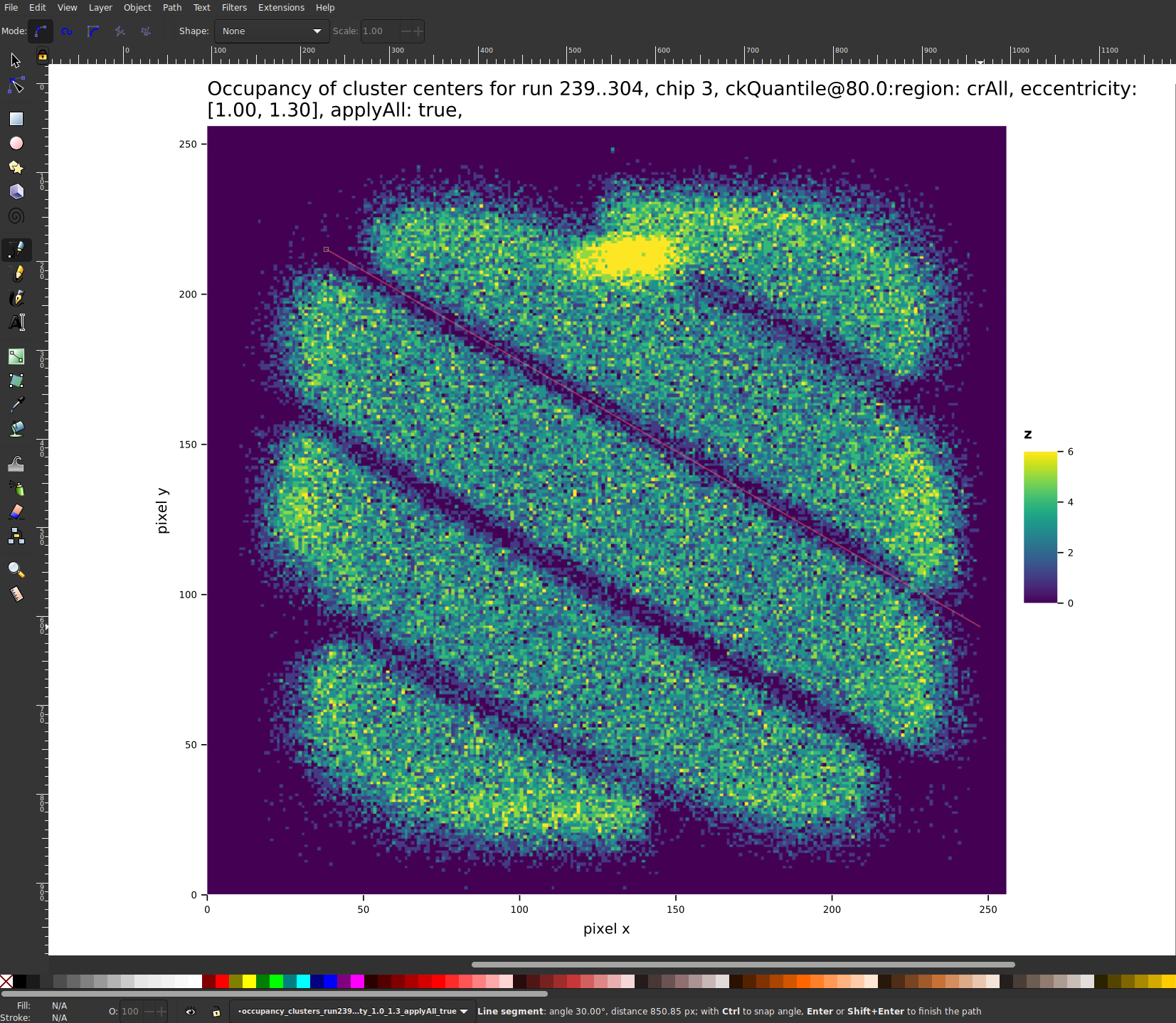
Need to check the number used in the raytracing code. There we have (also see discussion with Johanna in Discord):
    case wyKind
  of wy2017:
    result = degToRad(  10.8  )
  of wy2018:
    result = degToRad(  71.5  )
  of wyIAXO:
    result = degToRad(  20.0  ) #   who knows
so an angle of 71.5 (2018) and 10.8 (2017). Very different from the number we get in Inkscape based on the calibration runs.
She used the following plot:

to extract the angles.
The impact of this on the signal only depends on where the strongbacks are compared to the axion image.
Fig. 26 shows the axion image for the rotation of 71.5° (Johanna from X-ray finger) and fig. 27 shows the same for a rotation of 30° (our measurement). The 30° case matches nicely with the extraction of fig. 24.

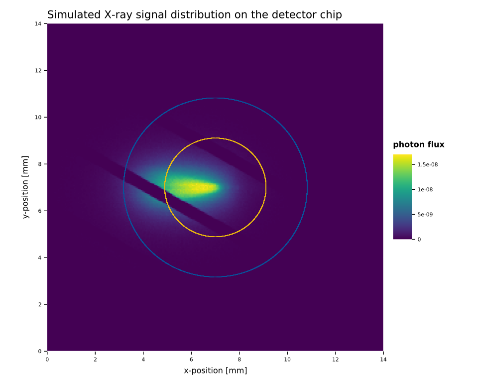
From here there are 2 things to do:
[X]reconstruct the X-ray finger runs & check the rotation of those again using the same occupancy plots as for the calibration runs.[X]compute the integrated signal for the 71.5°, 30° and 30°±0.5° cases and see how the signal differs. The latter will be the number for the systematic we'll use. We do that by just summing the raytracing output.
To do the latter, we need to add an option to write the CSV files in the raytracer first.
    import datamancer

proc print  (fname: string  ): float =
  let hmap = readCsv(fname)
  result = hmap[  "photon flux", float  ].sum
let f71 = print(  "/home/basti/org/resources/axion_images_systematics/axion_image_2018_71_5deg.csv"  )
let f30 = print(  "/home/basti/org/resources/axion_images_systematics/axion_image_2018_30deg.csv"  )
let f29 = print(  "/home/basti/org/resources/axion_images_systematics/axion_image_2018_29_5deg.csv"  )
let f31 = print(  "/home/basti/org/resources/axion_images_systematics/axion_image_2018_30_5deg.csv"  )

echo f71
echo f30
echo "Ratio : ", f30 / f71
echo "Ratio f29 / f31 ", f29 / f31
echo "Difference ", (  abs  (  1.0 - (f29/f30)  ) + abs  (  1.0 - (f31/f30)  )  ) / 2.0
Now on to the reconstruction of the X-ray finger run.
I copied the X-ray finger runs from tpc19 over to ./../CastData/data/XrayFingerRuns/. The run of interest is mainly the run 189, as it's the run done with the detector installed as in 2017/18 data taking.
    cd /dev/shm #   store here for fast access & temporary
cp ~/CastData/data/XrayFingerRuns/XrayFingerRun2018.tar.gz .
tar xzf XrayFingerRun2018.tar.gz
raw_data_manipulation -p Run_189_180420-09-53 --runType xray --out xray_raw_run189.h5
reconstruction -i xray_raw_run189.h5 --out xray_reco_run189.h5 #   make sure `config.toml` for reconstruction uses `default` clustering!
reconstruction -i xray_reco_run189.h5 --only_charge
reconstruction -i xray_reco_run189.h5 --only_gas_gain
reconstruction -i xray_reco_run189.h5 --only_energy_from_e
plotData --h5file xray_reco_run189.h5 --runType=rtCalibration -b bGgPlot --ingrid --occupancy --config plotData.toml
which gives us the following plot:

With many more plots here: ./../org/Figs/statusAndProgress/xrayFingerRun/run189/
Also see the relevant section in sec. 10.2.
Using TimepixAnalysis/Tools/printXyDataset we can now compute the
center of the X-ray finger run.
    cd ~/CastData/ExternCode/TimepixAnalysis/Tools/
./printXyDataset -f /dev/shm/xray_reco_run189.h5 -c 3 -r 189 \
                 --dset centerX --reco \
                 --cuts '("eccentricity", 0.9, 1.4)' \
                 --cuts '("centerX", 3.0, 11.0)' \
                 --cuts '("centerY", 3.0, 11.0)'

./printXyDataset -f /dev/shm/xray_reco_run189.h5 -c 3 -r 189 \
                 --dset centerY --reco \
                 --cuts '("eccentricity", 0.9, 1.4)' \
                 --cuts '("centerX", 3.0, 11.0)' \
                 --cuts '("centerY", 3.0, 11.0)'
So we get a mean of:
- centerX: 7.658
- centerY: 6.449
meaning we are ~0.5 mm away from the center in either direction. Given that there is distortion due to the magnet optic, uncertainty about the location of X-ray finger & emission characteristic, using a variation of 0.5mm seems reasonable.
This also matches more or less the laser alignment we did initially, see fig. 29.
- TODO Question about signal & window
One thing we currently do not take into account is that when varying the signal position using the nuisance parameters, we move the window strongback with the position…
In principle we're not allowed to do that. The strongbacks are part of the detector & not the signal (but are currently convolved into the image).
The strongback position depends on the detector mounting precision only.
So if the main peak was exactly on the strongback, we'd barely see anything!
13.11.4.5. Integration routines for nuisance parameters
For performance reasons we cannot integrate out the nuisance parameters using the most sophisticated algorithms. Maybe in the end we could assign a systematic by computing a few "accurate" integrations (e.g. integrating out \(ϑ_x\) and \(ϑ_y\)) with adaptive gauss and then with our chosen method and compare the result on the limit? Could just be a "total" uncertainty on the limit w/o changing any parameters.
13.11.5. Detector behavior [0/1] extended
[ ]drift in # hits in ⁵⁵Fe. "Adaptive gas gain" tries to minimize this, maybe variation of mean energy over time after application a measure for uncertainty? -> should mainly have an effect on software signal efficiency.- goes into S of limit likelihood (ε), which is currently assumed a constant number
[ ]veto random coincidences
13.11.5.1. Random coincidences
Come up with equation to compute rate of random coincidences.
Inputs:
- area of chip
- rate of cosmics
- shutter length
- physical time scale of background events
to compute rate of random coincidences.
Leads to effective reduction in live data taking time (increased dead time).
13.11.6. Background [0/2] extended
[ ]background interpolation- we already did: study of statistical uncertainty (both MC as well
as via error propagation)
[X]extract from error propagation code unclear what to do with these numbers!
- we already did: study of statistical uncertainty (both MC as well
as via error propagation)
[ ]septem veto can suffer from uncertainties due to possible random coincidences of events on outer chip that veto a center event, which are not actually correlated. In our current application of it, this implies a) a lower background rate, but b) a lower software signal efficiency as we might also remove real photons. So its effect is on ε as ell.[ ]think about random coincidences, derive some formula similar to lab course to compute chance
13.11.6.1. Background interpolation [0/1]
Ref: 13.10.8.4
and ntangle this file and run
/tmp/background_interpolation_error_propagation.nim for the
background interpolation with Measuremancer error propagation.
For an input of 8 clusters in a search radius around a point we get
numbers such as:
Normalized value (gauss) : 6.08e-06 ± 3.20e-06 CentiMeter⁻²•Second⁻¹
so an error that is almost 50% of the input.
However, keep in mind that this is for a small area around the specific point. Just purely from Poisson statistics we expect an uncertainty of 2.82 for 8 events \[ ΔN = √8 = 2.82 \]
As such this makes sense (the number is larger due to the gaussian
nature of the distance calculation etc.) and just being a weighted sum
of 1 ± 1 terms error propagated.
If we compute the same for a larger number of points, the error should go down, which can be seen comparing fig. 18 with fig. 19 (where the latter has artificially increased statistics).
As this is purely a statistical effect, I'm not sure how to quantify any kind of systematic errors.
The systematics come into play, due to the:
- choice of radius & sigma
- choice of gaussian weighting
- choice of "energy radius"
[ ]look at background interpolation uncertainty section linked above. Modify to also include a section about a flat model that varies the different parameters going into the interpolation.[ ]use existing code to compute a systematic based on the kind of background model. Impact of background hypothesis?
13.11.7. Energy calibration, likelihood method [0/1] extended
[ ]the energy calibration as a whole has many uncertainties (due to detector variation, etc.)- gas gain time binning:
[ ]compute everything up to background rate for no time binning, 90 min and maybe 1 or 2 other values. Influence on σb is the change in background that we see from this (will be a lot of work, but useful to make things more reproducible).
[ ]compute energy of 55Fe peaks after energy calibration. Variation gives indication for systematic influence.
- gas gain time binning:
13.11.7.1. Gas gain time binning
We need to investigate the impact of the gas gain binning on the background rate. How do we achieve that?
Simplest approach:
- Compute gas gain slices for different cases (no binning, 30 min binning, 90 min binning, 240 min binning ?)
- calculate energy based on the used gas gain binning
- compute the background rate for each case
- compare amount of background after that.
Question: Do we need to recompute the gas gain for the calibration data as well? Yes, as the gas gain slices directly go into the 'gain fit' that needs to be done in order to compute the energy for any cluster.
So, the whole process is only made complicated by the fact that we
need to change the config.toml file in between runs. In the future
this should be a CL argument. For the time being, we can use the same
approach as in
/home/basti/CastData/ExternCode/TimepixAnalysis/Tools/backgroundRateDifferentEffs/backgroundRateDifferentEfficiencies.nim
where we simply read the toml file, rewrite the single line and write
it back.
Let's write a script that does mainly steps 1 to 3 for us.
    import shell, strformat, strutils, sequtils, os

#   an interval of 0 implies _no_ gas gain interval, i.e. full run
const intervals = [  0, 30, 90, 240  ]
const Tmpl = "  $#  Runs  $#  _Reco.h5"
const Path = "/home/basti/CastData/data/systematics/"
const TomlFile = "/home/basti/CastData/ExternCode/TimepixAnalysis/Analysis/ingrid/config.toml"

proc rewriteToml  (path: string, interval: int  ) =
  ## rewrites the given TOML file in the `  path  ` to use the `  interval  `
  ## instead of the existing value
  var data = readFile  (path).splitLines
  for l in mitems  (data):
    if interval == 0 and l.startsWith(  "fullRunGasGain"  ):
      l = "fullRunGasGain = true"
    elif interval != 0 and l.startsWith(  "fullRunGasGain"  ):
      l = "fullRunGasGain = false"
    elif interval != 0 and l.startsWith(  "gasGainInterval"  ):
      l = "gasGainInterval = " & $interval
  writeFile  (path, data.join(  "\n"  )  )

proc computeGasGainSlices  (fname: string, interval: int  ) =
  let (res, err, code) = shellVerboseErr:
    one:
      cd ~/CastData/data/systematics
      reconstruction ($fname) "--only_gas_gain"
  if code != 0:
    raise newException  (  Exception, "Error calculating gas gain for interval " & $interval)

proc computeGasGainFit  (fname: string, interval: int  ) =
  let (res, err, code) = shellVerboseErr:
    one:
      cd ~/CastData/data/systematics
      reconstruction ($fname) "--only_gain_fit"
  if code != 0:
    raise newException  (  Exception, "Error calculating gas gain fit for interval " & $interval)

proc computeEnergy  (fname: string, interval: int  ) =
  let (res, err, code) = shellVerboseErr:
    one:
      cd ~/CastData/data/systematics
      reconstruction ($fname) "--only_energy_from_e"
  if code != 0:
    raise newException  (  Exception, "Error calculating energy for interval " & $interval)

proc computeLikelihood  (f, outName: string, interval: int  ) =
  let args = { "--altCdlFile" : "~/CastData/data/CDL_2019/calibration-cdl-2018.h5",
               "--altRefFile" : "~/CastData/data/CDL_2019/XrayReferenceFile2018.h5",
               "--cdlYear" : "2018",
               "--region" : "crGold"  }
  let argStr = args.mapIt(it[  0  ] & " " & it[  1  ]  ).join(  " "  )
  let (res, err, code) = shellVerboseErr:
    one:
      cd ~/CastData/data/systematics
      likelihood ($f) "--h5out" ($outName) ($argStr)
  if code != 0:
    raise newException  (  Exception, "Error computing likelihood cuts for interval " & $interval)

#  proc plotBackgroundRate(f1, f2: string, eff: float) =
#    let suffix = &"_eff_{eff}"
#    let (res, err, code) = shellVerboseErr:
#      one:
#        cd ~/CastData/ExternCode/TimepixAnalysis/Plotting/plotBackgroundRate
#        ./plotBackgroundRate ($f1) ($f2) "--suffix" ($suffix)
#        ./plotBackgroundRate ($f1) ($f2) "--separateFiles --suffix" ($suffix)
#    if code != 0:
#      raise newException(Exception, "Error plotting background rate for eff " & $eff)

let years = [  2017, 2018  ]
let calibs = years.mapIt(  Tmpl % [  "Calibration", $it]  )
let backs = years.mapIt(  Tmpl % [  "Data", $it]  )

copyFile(  TomlFile, "/tmp/toml_file.backup"  )
for interval in intervals:
  ## rewrite toml file
  rewriteToml(  TomlFile, interval)
  ## compute new gas gain for new interval for all files
  for f in concat(calibs, backs):
    computeGasGainSlices(f, interval)
  ## use gas gain slices to compute gas gain fit
  for f in calibs:
    computeGasGainFit(f, interval)
  ## compute energy based on new gain fit
  for f in concat(calibs, backs):
    computeEnergy(f, interval)
  ## compute likelihood based on new energies
  var logFs = newSeq  [  string  ]()
  for b in backs:
    let yr = if "2017" in b: "2017" else: "2018"
    let fname = &"out/lhood_{yr}_interval_{interval}.h5"
    logFs.add fname
    ## XXX: need to redo likelihood computation!!
    computeLikelihood(b, fname, interval)
## plot background rate for all combined? or just plot cluster centers? can all be done later...
#  plotBackgroundRate(log, eff)
    import shell, strformat, strutils, sequtils, os

#   an interval of 0 implies _no_ gas gain interval, i.e. full run
const intervals = [  0, 30, 90, 240  ]
const Tmpl = "  $#  Runs  $#  _Reco.h5"
echo (  Tmpl % [  "Data", "2017"  ]  ).extractFilename
The resulting files are found in ./../CastData/data/systematics/out/ or ./../CastData/data/systematics/ on my laptop.
Let's extract the number of clusters found on the center chip (gold region) for each of the intervals:
    cd ~/CastData/data/systematics
for i in 0 30 90 240
  do   echo Inteval: $i
     extractClusterInfo -f lhood_2017_interval_$i.h5 --short --region crGold
     extractClusterInfo -f lhood_2018_interval_$i.h5 --short --region crGold
done
The numbers pretty much speak for themselves.
    let nums = { 0 : 497 + 244,
             30 : 499 + 244,
             90 : 500 + 243,
             240 : 497 + 244 }
#   reference is 90
let num90 = nums[  2  ][  1  ]
var minVal = Inf
var maxVal = 0.0
for num in nums:
  let rat = num[  1  ] / num90
  echo "Ratio of ", num, " = ", rat
  minVal = min  (minVal, rat)
  maxVal = max  (maxVal, rat)
echo "Deviation: ", maxVal - minVal
NOTE: The one 'drawback' of this approach taken here is the following: the CDL data was not reconstructed using the changed gas gain data. However that is much less important, as we assume constant gain over the CDL runs anyway more or less / want to pick the most precise description of our data!
13.11.7.2. Interpolation of reference distributions (CDL morphing) [/]
We already did the study of the variation in the interpolation for the reference distributions. To estimate the systematic uncertainty related to that, we should simply look at the computation of the "intermediate" distributions again and compare the real numbers to the interpolated ones. The deviation can be done per bin. The average & some quantiles should be a good number to refer to as a systematic.
The cdlMorphing tool
./../CastData/ExternCode/TimepixAnalysis/Tools/cdlMorphing/cdlMorphing.nim
is well suited to this. We will compute the difference between the
morphed and real data for each bin & sum the squares for each
target/filter (those that are morphed, so not the outer two of
course).
Running the tool now yields the following output:
  Target/Filter: Cu-EPIC-0.9kV = 0.0006215219861090395
Target/Filter: Cu-EPIC-2kV = 0.0007052150065674744
Target/Filter: Al-Al-4kV = 0.001483398679126846
Target/Filter: Ag-Ag-6kV = 0.001126063558474516
Target/Filter: Ti-Ti-9kV = 0.0006524420692883554
Target/Filter: Mn-Cr-12kV = 0.0004757207676502019
Mean difference 0.0008440603445360723
So we really have a miniscule difference there.
[ ]also compute the background rate achieved using no CDL morphing vs using it.
13.11.7.3. Energy calibration [/]
[ ]compute peaks of 55Fe energy. What is variation?
13.11.7.4. Software efficiency systematic [/]
In order to guess at the systematic uncertainty of the software efficiency, we can push all calibration data through the likelihood cuts and evaluate the real efficiency that way.
This means the following:
- compute likelihood values for all calibration runs
- for each run, remove extreme outliers using rough RMS transverse & eccentricity cuts
- filter to 2 energies (essentially a secondary cut), the photopeak and escape peak
- for each peak, push through likelihood cut. # after / # before is software efficiency at that energy
The variation we'll see over all runs tells us something about the systematic uncertainty & potential bias.
UPDATE: The results presented below the code were computed with the
code snippet here as is (and multiple arguments of course, check
zsh_history at home for details). A modified version now also lives
at
./../CastData/ExternCode/TimepixAnalysis/Tools/determineEffectiveEfficiency.nim
[ ]REMOVE THE PIECE OF CODE HERE, REPLACE BY CALL TO ABOVE!
UPDATE2 : While working on the below code for
the script mentioned in the first update, I noticed a bug in the
filterEvents function:
        of "Escapepeak":
        let dset = 5.9.toRefDset()
        let xrayCuts = xrayCutsTab[dset]
        result.add applyFilters(df)
      of "Photopeak":
        let dset = 2.9.toRefDset()
        let xrayCuts = xrayCutsTab[dset]
        result.add applyFilters(df)
the energies are exchanged and applyFilters is applied to df and
not subDf as it should here!
[ ]Investigate the effect for the systematics of CAST! -> : I just had a short look at this. It seems like this is the correct output:
DataFrame with 3 columns and 67 rows: Idx Escapepeak Photopeak RunNumber dtype: float float int 0 0.6579 0.7542 83 1 0.6452 0.787 88 2 0.6771 0.7667 93 3 0.7975 0.7599 96 4 0.799 0.7605 102 5 0.8155 0.7679 108 6 0.7512 0.7588 110 7 0.8253 0.7769 116 8 0.7766 0.7642 118 9 0.7752 0.7765 120 10 0.7556 0.7678 122 11 0.7788 0.7711 126 12 0.7749 0.7649 128 13 0.8162 0.7807 145 14 0.8393 0.7804 147 15 0.7778 0.78 149 16 0.8153 0.778 151 17 0.7591 0.7873 153 18 0.8229 0.7819 155 19 0.8341 0.7661 157 20 0.7788 0.7666 159 21 0.7912 0.7639 161 22 0.8041 0.7675 163 23 0.7884 0.777 165 24 0.8213 0.7791 167 25 0.7994 0.7833 169 26 0.8319 0.7891 171 27 0.8483 0.7729 173 28 0.7973 0.7733 175 29 0.834 0.7771 177 30 0.802 0.773 179 31 0.7763 0.7687 181 32 0.8061 0.766 183 33 0.7916 0.7799 185 34 0.8131 0.7745 187 35 0.8366 0.8256 239 36 0.8282 0.8035 241 37 0.8072 0.8045 243 38 0.851 0.8155 245 39 0.7637 0.8086 247 40 0.8439 0.8135 249 41 0.8571 0.8022 251 42 0.7854 0.7851 253 43 0.8159 0.7843 255 44 0.815 0.7827 257 45 0.8783 0.8123 259 46 0.8354 0.8094 260 47 0.8 0.789 262 48 0.8038 0.8097 264 49 0.7926 0.7937 266 50 0.8275 0.7961 269 51 0.8514 0.8039 271 52 0.8089 0.7835 273 53 0.8134 0.7789 275 54 0.8168 0.7873 277 55 0.8198 0.7886 280 56 0.8447 0.7833 282 57 0.7876 0.7916 284 58 0.8093 0.8032 286 59 0.7945 0.8059 288 60 0.8407 0.7981 290 61 0.7824 0.78 292 62 0.7885 0.7869 294 63 0.7933 0.7823 296 64 0.837 0.7834 300 65 0.7594 0.7826 302 66 0.8333 0.7949 304
Std Escape = 0.04106537728575545 Std Photo = 0.01581231947284212 Mean Escape = 0.8015071105396809 Mean Photo = 0.7837728948033928
So a bit worse than initially thought…
    import std / [os, strutils, random, sequtils, stats, strformat]
import nimhdf5, cligen
import numericalnim except linspace


import ingrid / private / [likelihood_utils, hdf5_utils, ggplot_utils, geometry, cdl_cuts]
import ingrid / calibration
import ingrid / calibration / [fit_functions]
import ingrid / ingrid_types
import ingridDatabase / [databaseRead, databaseDefinitions, databaseUtils]

#   cut performed regardless of logL value on the data, since transverse
#   rms > 1.5 cannot be a physical photon, due to diffusion in 3cm drift
#   distance
const RmsCleaningCut = 1.5

let CdlFile = "/home/basti/CastData/data/CDL_2019/calibration-cdl-2018.h5"
let RefFile = "/home/basti/CastData/data/CDL_2019/XrayReferenceFile2018.h5"

proc drawNewEvent  (rms, energy: seq  [  float  ]  ): int =
  let num = rms.len - 1
  var idx = rand(num)
  while rms[idx] >= RmsCleaningCut or
        (energy[idx] <= 4.5 or energy[idx] >= 7.5  ):
    idx = rand(num)
  result = idx

proc computeEnergy  (h5f: H5File, pix: seq  [  Pix  ], group: string, a, b, c, t, bL, mL: float  ): float =
  let totalCharge = pix.mapIt(calibrateCharge(it.ch.float, a, b, c, t)  ).sum
  #   compute mean of all gas gain slices in this run (most sensible)
  let gain = h5f[group / "chip_3/gasGainSlices", GasGainIntervalResult  ].mapIt(it.G  ).mean
  let calibFactor = linearFunc(@[bL, mL], gain) * 1e-6
  #   now calculate energy for all hits
  result = totalCharge * calibFactor

proc generateFakeData  (h5f: H5File, nFake: int, energy = 3.0  ): DataFrame =
  ## For each run generate `  nFake  ` fake events
  let refSetTuple = readRefDsets(  RefFile, yr2018)
  result = newDataFrame()
  for (num, group) in runs(h5f):
    #   first read all x / y / tot data
    echo "Run number: ", num
    let xs = h5f[group / "chip_3/x", special_type(  uint8  ), uint8  ]
    let ys = h5f[group / "chip_3/y", special_type(  uint8  ), uint8  ]
    let ts = h5f[group / "chip_3/ToT", special_type(  uint16  ), uint16  ]
    let rms = h5f[group / "chip_3/rmsTransverse", float  ]
    let cX = h5f[group / "chip_3/centerX", float  ]
    let cY = h5f[group / "chip_3/centerY", float  ]
    let energyInput = h5f[group / "chip_3/energyFromCharge", float  ]
    let chipGrp = h5f[  (group / "chip_3"  ).grp_str]
    let chipName = chipGrp.attrs[  "chipName", string  ]
    #   get factors for charge calibration
    let (a, b, c, t) = getTotCalibParameters(chipName, num)
    #   get factors for charge / gas gain fit
    let (bL, mL) = getCalibVsGasGainFactors(chipName, num, suffix = $gcIndividualFits)
    var count = 0
    var evIdx = 0

    when false:
      for i in 0 ..< xs.len:
        if xs[i].len < 150 and energyInput[i] > 5.5:
          #   recompute from data
          let pp = toSeq(  0 ..< xs[i].len  ).mapIt(  (x: xs[i][it], y: ys[i][it], ch: ts[i][it]  )  )
          let newEnergy = h5f.computeEnergy(pp, group, a, b, c, t, bL, mL)
          echo "Length ", xs[i].len , " w/ energy ", energyInput[i], " recomp ", newEnergy
          let df = toDf(  {  "x" : pp.mapIt(it.x.int  ), "y" : pp.mapIt(it.y.int  ), "ch" : pp.mapIt(it.ch.int  )  }  )
          ggplot(df, aes(  "x", "y", color = "ch"  )  ) +
            geom_point() +
            ggtitle(  "funny its real"  ) +
            ggsave(  "/tmp/fake_event_" & $i & ".pdf"  )
          sleep(  200  )
      if true: quit  ()

    #   to store fake data
    var energies = newSeqOfCap[  float  ](nFake)
    var logLs = newSeqOfCap[  float  ](nFake)
    var rmss = newSeqOfCap[  float  ](nFake)
    var eccs = newSeqOfCap[  float  ](nFake)
    var ldivs = newSeqOfCap[  float  ](nFake)
    var frins = newSeqOfCap[  float  ](nFake)
    var cxxs = newSeqOfCap[  float  ](nFake)
    var cyys = newSeqOfCap[  float  ](nFake)
    var lengths = newSeqOfCap[  float  ](nFake)
    while count < nFake:
      #   draw index from to generate a fake event
      evIdx = drawNewEvent(rms, energyInput)
      #   draw number of fake pixels
      #   compute ref # pixels for this event taking into account possible double counting etc.
      let basePixels = (energy / energyInput[evIdx] * xs[evIdx].len.float  )
      let nPix = round(basePixels + gauss(sigma = 10.0  )  ).int  #   ~115 pix as reference in 3 keV (26 eV), draw normal w/10 around
      if nPix < 4:
        echo "Less than 4 pixels: ", nPix, " skipping"
        continue
      var pix = newSeq  [  Pix  ](nPix)
      var seenPix: set  [  uint16  ] = {}
      let evNumPix = xs[evIdx].len

      if nPix >= evNumPix:
        echo "More pixels to draw than available! ", nPix, " vs ", evNumPix, ", skipping!"
        continue
      if not inRegion(cX[evIdx], cY[evIdx], crSilver):
        echo "Not in silver region. Not a good basis"
        continue

      var pIdx = rand(evNumPix - 1  )
      for j in 0 ..< nPix:
        #   draw pix index
        while pIdx.uint16 in seenPix:
          pIdx = rand(evNumPix - 1  )
        seenPix.incl pIdx.uint16
        pix[j] = (x: xs[evIdx][pIdx], y: ys[evIdx][pIdx], ch: ts[evIdx][pIdx]  )
      #   now draw
      when false:
        let df = toDf(  {  "x" : pix.mapIt(it.x.int  ), "y" : pix.mapIt(it.y.int  ), "ch" : pix.mapIt(it.ch.int  )  }  )
        ggplot(df, aes(  "x", "y", color = "ch"  )  ) +
          geom_point() +
          ggsave(  "/tmp/fake_event.pdf"  )
        sleep(  200  )

      #   reconstruct event
      let inp = (pixels: pix, eventNumber: 0, toa: newSeq  [  uint16  ](), toaCombined: newSeq  [  uint64  ]()  )
      let recoEv = recoEvent(inp, -1,
                             num, searchRadius = 50,
                             dbscanEpsilon = 65,
                             clusterAlgo = caDefault)
      if recoEv.cluster.len > 1 or recoEv.cluster.len == 0:
        echo "Found more than 1 or 0 cluster! Skipping"
        continue
      #   compute charge
      let energy = h5f.computeEnergy(pix, group, a, b, c, t, bL, mL)

      #   puhhh, now the likelihood...
      let ecc = recoEv.cluster[  0  ].geometry.eccentricity
      let ldiv = recoEv.cluster[  0  ].geometry.lengthDivRmsTrans
      let frin = recoEv.cluster[  0  ].geometry.fractionInTransverseRms
      let logL = calcLikelihoodForEvent(energy,
                                        ecc,
                                        ldiv,
                                        frin,
                                        refSetTuple)
      #   finally done
      energies.add energy
      logLs.add logL
      rmss.add recoEv.cluster[  0  ].geometry.rmsTransverse
      eccs.add ecc
      ldivs.add ldiv
      frins.add frin
      cxxs.add recoEv.cluster[  0  ].centerX
      cyys.add recoEv.cluster[  0  ].centerY
      lengths.add recoEv.cluster[  0  ].geometry.length
      inc count
    let df = toDf(  { "energyFromCharge" : energies,
                    "likelihood" : logLs,
                    "runNumber" : num,
                    "rmsTransverse" : rmss,
                    "eccentricity" : eccs,
                    "lengthDivRmsTrans" : ldivs,
                    "centerX" : cxxs,
                    "centerY" : cyys,
                    "length" : lengths,
                    "fractionInTransverseRms" : frins }  )
    result.add df

proc applyLogLCut  (df: DataFrame, cutTab: CutValueInterpolator  ): DataFrame =
  result = df.mutate(f{  float: "passLogL?" ~ (  block:
                                               #  echo "Cut value: ", cutTab[idx(igEnergyFromCharge.toDset())], " at dset ", toRefDset(idx(igEnergyFromCharge.toDset())), " at energy ", idx(igEnergyFromCharge.toDset())
                                               idx(igLikelihood.toDset()  ) < cutTab[idx(igEnergyFromCharge.toDset()  )  ]  )  }  )

proc readRunData  (h5f: H5File  ): DataFrame =
  result = h5f.readDsets(chipDsets =
    some(  (chip: 3,
          dsets: @[igEnergyFromCharge.toDset(),
                   igRmsTransverse.toDset(),
                   igLengthDivRmsTrans.toDset(),
                   igFractionInTransverseRms.toDset(),
                   igEccentricity.toDset(),
                   igCenterX.toDset(),
                   igCenterY.toDset(),
                   igLength.toDset(),
                   igLikelihood.toDset()  ]  )  )  )

proc filterEvents  (df: DataFrame, energy: float = Inf  ): DataFrame =
  let xrayCutsTab   {.global.} = getXrayCleaningCuts()
  template applyFilters  (dfI: untyped  ): untyped {.dirty.} =
    let minRms = xrayCuts.minRms
    let maxRms = xrayCuts.maxRms
    let maxLen = xrayCuts.maxLength
    let maxEcc = xrayCuts.maxEccentricity
    dfI.filter(f{  float -> bool: idx(igRmsTransverse.toDset()  ) < RmsCleaningCut and
      inRegion(idx(  "centerX"  ), idx(  "centerY"  ), crSilver) and
      idx(  "rmsTransverse"  ) >= minRms and
      idx(  "rmsTransverse"  ) <= maxRms and
      idx(  "length"  ) <= maxLen and
      idx(  "eccentricity"  ) <= maxEcc
    }  )
  if "Peak" in df:
    doAssert classify(energy) == fcInf
    result = newDataFrame()
    for (tup, subDf) in groups(df.group_by(  "Peak"  )  ):
      case tup[  0  ][  1  ].toStr
      of "Escapepeak":
        let dset = 5.9.toRefDset()
        let xrayCuts = xrayCutsTab[dset]
        result.add applyFilters(df)
      of "Photopeak":
        let dset = 2.9.toRefDset()
        let xrayCuts = xrayCutsTab[dset]
        result.add applyFilters(df)
      else: doAssert false, "Invalid name"
  else:
    doAssert classify(energy) != fcInf
    let dset = energy.toRefDset()
    let xrayCuts = xrayCutsTab[dset]
    result = applyFilters(df)

proc splitPeaks  (df: DataFrame  ): DataFrame =
  let eD = igEnergyFromCharge.toDset()
  result = df.mutate(f{  float -> string: "Peak" ~ (
    if idx(eD) < 3.5 and idx(eD) > 2.5:
      "Escapepeak"
    elif idx(eD) > 4.5 and idx(eD) < 7.5:
      "Photopeak"
    else:
      "None"  )  }  )
    .filter(f{`Peak` != "None"  }  )

proc handleFile  (fname: string, cutTab: CutValueInterpolator  ): DataFrame =
  ## Given a single input file, performs application of the likelihood cut for all
  ## runs in it, split by photo & escape peak. Returns a DF with column indicating
  ## the peak, energy of each event & a column whether it passed the likelihood cut.
  ## Only events that are pass the input cuts are stored.
  let h5f = H5open  (fname, "r"  )
  randomize(  423  )
  result = newDataFrame()
  let data = h5f.readRunData()
    .splitPeaks()
    .filterEvents()
    .applyLogLCut(cutTab)
  result.add data
  when false:
    ggplot(  result, aes(  "energyFromCharge"  )  ) +
      geom_histogram(bins = 200  ) +
      ggsave(  "/tmp/ugl.pdf"  )
  discard h5f.close  ()

proc handleFakeData  (fname: string, energy: float, cutTab: CutValueInterpolator  ): DataFrame =
  let h5f = H5open  (fname, "r"  )
  var data = generateFakeData(h5f, 5000, energy = energy)
    .filterEvents(energy)
    .applyLogLCut(cutTab)
  result = data
  discard h5f.close  ()

proc getIndices  (dset: string  ): seq  [  int  ] =
  result = newSeq  [  int  ]()
  applyLogLFilterCuts(  CdlFile, RefFile, dset, yr2018, igEnergyFromCharge):
    result.add i

proc plotRefHistos  (df: DataFrame, energy: float, cutTab: CutValueInterpolator,
                   dfAdditions: seq  [  tuple  [name: string, df: DataFrame  ]  ] = @[]  ) =
  #   map input fake energy to reference dataset
  let grp = energy.toRefDset()

  let passedInds = getIndices(grp)
  let h5f = H5open  (  RefFile, "r"  )
  let h5fC = H5open  (  CdlFile, "r"  )
  const xray_ref = getXrayRefTable()
  #  for (i, grp) in pairs(xray_ref):

  var dfR = newDataFrame()
  for dset in IngridDsetKind:
    try:
      let d = dset.toDset()
      if d notin df: continue #   skip things not in input
      ## first read data from CDL file (exists for sure)
      ## extract all CDL data that passes the cuts used to generate the logL histograms
      var cdlFiltered = newSeq  [  float  ](passedInds.len  )
      let cdlRaw = h5fC[cdlGroupName(grp, "2019", d), float  ]
      for i, idx in passedInds:
        cdlFiltered[i] = cdlRaw[idx]
      echo "Total number of elements ", cdlRaw.len, " filtered to ", passedInds.len
      dfR[d] = cdlFiltered
      ## now read histograms from RefFile, if they exist (not all datasets do)
      if grp / d in h5f:
        let dsetH5 = h5f[  (grp / d).dset_str]
        let (bins, data) = dsetH5[  float  ].reshape2D(dsetH5.shape).split(  Seq2Col  )
        let fname = &"/tmp/{grp}_{d}_energy_{energy:.1f}.pdf"
        echo "Storing histogram in : ", fname
        #   now add fake data
        let dataSum = simpson(data, bins)
        let refDf = toDf(  {  "bins" : bins, "data" : data}  )
          .mutate(f{  "data" ~ `data` / dataSum}  )
        let df = df.filter(f{  float: idx(d) <= bins[^1  ]  }  )
        ggplot(refDf, aes(  "bins", "data"  )  ) +
          geom_histogram(stat = "identity", hdKind = hdOutline, alpha = 0.5  ) +
          geom_histogram(data = df, aes = aes(d), bins = 200, alpha = 0.5,
                         fillColor = "orange", density = true, hdKind = hdOutline) +
          ggtitle(&"{d}. Orange: fake data from 'reducing' 5.9 keV data @ {energy:.1f}. Black: CDL ref {grp}"  ) +
          ggsave(fname, width = 1000, height = 600  )
    except AssertionError:
      continue

  #   get effect of logL cut on CDL data
  dfR = dfR.applyLogLCut(cutTab)
  var dfs = @[  (  "Fake", df), (  "Real", dfR)  ]
  if dfAdditions.len > 0:
    dfs = concat(dfs, dfAdditions)
  var dfPlot = bind_rows(dfs, "Type"  )
  echo "Rough filter removes: ", dfPlot.len
  dfPlot = dfPlot.filter(f{`lengthDivRmsTrans` <= 50.0 and `eccentricity` <= 5.0  }  )
  echo "To ", dfPlot.len, " elements"
  ggplot(dfPlot, aes(  "lengthDivRmsTrans", "fractionInTransverseRms", color = "eccentricity"  )  ) +
    facet_wrap(  "Type"  ) +
    geom_point(size = 1.0, alpha = 0.5  ) +
    ggtitle(&"Fake energy: {energy:.2f}, CDL dataset: {grp}"  ) +
    ggsave(&"/tmp/scatter_colored_fake_energy_{energy:.2f}.png", width = 1200, height = 800  )

  #   plot likelihood histos
  ggplot(dfPlot, aes(  "likelihood", fill = "Type"  )  ) +
    geom_histogram(bins = 200, alpha = 0.5, hdKind = hdOutline) +
    ggtitle(&"Fake energy: {energy:.2f}, CDL dataset: {grp}"  ) +
    ggsave(&"/tmp/histogram_fake_energy_{energy:.2f}.pdf", width = 800, height = 600  )

  discard h5f.close  ()
  discard h5fC.close  ()


  echo "DATASET : ", grp, "--------------------------------------------------------------------------------"
  echo "Efficiency of logL cut on filtered CDL data (should be 80%!) = ", dfR.filter(f{idx(  "passLogL?"  ) == true  }  ).len.float / dfR.len.float
  echo "Elements passing using `passLogL?` ", dfR.filter(f{idx(  "passLogL?"  ) == true  }  ).len, " vs total ", dfR.len
  let (hist, bins) = histogram(dfR[  "likelihood", float  ].toRawSeq, 200, (  0.0, 30.0  )  )
  ggplot(toDf(  {  "Bins" : bins, "Hist" : hist}  ), aes(  "Bins", "Hist"  )  ) +
    geom_histogram(stat = "identity"  ) +
    ggsave(  "/tmp/usage_histo_" & $grp & ".pdf"  )
  let cutval = determineCutValue(hist, eff = 0.8  )
  echo "Effficiency from `determineCutValue? ", bins[cutVal]

proc main  (files: seq  [  string  ], fake = false, real = false, refPlots = false,
          energies: seq  [  float  ] = @[]  ) =
  ## given the input files of calibration runs, walks all files to determine the
  ## 'real' software efficiency for them & generates a plot
  let cutTab = calcCutValueTab(  CdlFile, RefFile, yr2018, igEnergyFromCharge)
  var df = newDataFrame()
  if real and not fake:
    for f in files:
      df.add handleFile(f, cutTab)
    var effEsc = newSeq  [  float  ]()
    var effPho = newSeq  [  float  ]()
    var nums = newSeq  [  int  ]()
    for (tup, subDf) in groups(df.group_by(@[  "runNumber", "Peak"  ]  )  ):
      echo "------------------"
      echo tup
      #  echo subDf
      let eff = subDf.filter(f{idx(  "passLogL?"  ) == true  }  ).len.float / subDf.len.float
      echo "Software efficiency: ", eff
      if tup[  1  ][  1  ].toStr == "Escapepeak":
        effEsc.add eff
      elif tup[  1  ][  1  ].toStr == "Photopeak":
        effPho.add eff
        #   only add in one branch
        nums.add tup[  0  ][  1  ].toInt
      echo "------------------"
    let dfEff = toDf(  {  "Escapepeak" : effEsc, "Photopeak" : effPho, "RunNumber" : nums}  )
    echo dfEff.pretty(-1  )
    let stdEsc = effEsc.standardDeviationS
    let stdPho = effPho.standardDeviationS
    let meanEsc = effEsc.mean
    let meanPho = effPho.mean
    echo "Std Escape = ", stdEsc
    echo "Std Photo = ", stdPho
    echo "Mean Escape = ", meanEsc
    echo "Mean Photo = ", meanPho
    ggplot(dfEff.gather(  [  "Escapepeak", "Photopeak"  ], "Type", "Value"  ), aes(  "Value", fill = "Type"  )  ) +
      geom_histogram(bins = 20, hdKind = hdOutline, alpha = 0.5  ) +
      ggtitle(&"σ_escape = {stdEsc:.4f}, μ_escape = {meanEsc:.4f}, σ_photo = {stdPho:.4f}, μ_photo = {meanPho:.4f}"  ) +
      ggsave(  "/tmp/software_efficiencies_cast_escape_photo.pdf", width = 800, height = 600  )

    for (tup, subDf) in groups(df.group_by(  "Peak"  )  ):
      case tup[  0  ][  1  ].toStr
      of "Escapepeak": plotRefHistos(df, 2.9, cutTab)
      of "Photopeak": plotRefHistos(df, 5.9, cutTab)
      else: doAssert false, "Invalid data: " & $tup[  0  ][  1  ].toStr
  if fake and not real:
    var effs = newSeq  [  float  ]()
    for e in energies:
      if e > 5.9:
        echo "Warning: energy above 5.9 keV not allowed!"
        return
      df = newDataFrame()
      for f in files:
        df.add handleFakeData(f, e, cutTab)
      plotRefHistos(df, e, cutTab)

      echo "Done generating for energy ", e
      effs.add  (df.filter(f{idx(  "passLogL?"  ) == true  }  ).len.float / df.len.float  )
    let dfL = toDf(  {  "Energy" : energies, "Efficiency" : effs}  )
    echo dfL
    ggplot(dfL, aes(  "Energy", "Efficiency"  )  ) +
      geom_point() +
      ggtitle(  "Software efficiency from 'fake' events"  ) +
      ggsave(  "/tmp/fake_software_effs.pdf"  )
  if fake and real:
    doAssert files.len == 1, "Not more than 1 file supported!"
    let f = files[  0  ]
    let dfCast = handleFile(f, cutTab)

    for (tup, subDf) in groups(dfCast.group_by(  "Peak"  )  ):
      case tup[  0  ][  1  ].toStr
      of "Escapepeak":
        plotRefHistos(handleFakeData(f, 2.9, cutTab), 2.9, cutTab, @[  (  "CAST", subDf)  ]  )
      of "Photopeak":
        plotRefHistos(handleFakeData(f, 5.9, cutTab), 5.9, cutTab, @[  (  "CAST", subDf)  ]  )
      else: doAssert false, "Invalid data: " & $tup[  0  ][  1  ].toStr

  #  if refPlots:
  #    plotRefHistos()

when isMainModule:
  dispatch main
UPDATE : The discussion about the results of the above code here is limited to the results relevant for the systematic of the software efficiency. For the debugging of the unexpected software efficiencies computed for the calibration photo & escape peaks, see section ./../org/Doc/StatusAndProgress.html.
After the debugging session trying to figure out why the hell the software efficiency is so different, here are finally the results of this study.
The software efficiencies for the escape & photopeak energies from the calibration data at CAST are determined as follows:
- filter to events with
rmsTransverse<= 1.5 - filter to events within the silver region
- filter to events passing the 'X-ray cuts'
- for escape & photopeak each filter to energies of 1 & 1.5 keV around the peak
The remaining events are then used as the "basis" for the evaluation. From here the likelihood cut method is applied to all clusters. In the final step the ratio of clusters passing the logL cut over all clusters is computed, which gives the effective software efficiency for the data.
For all 2017 and 2018 runs this gives:
  Dataframe with 3 columns and 67 rows:
           Idx    Escapepeak     Photopeak     RunNumber
        dtype:         float         float           int
             0        0.6886         0.756            83
             1        0.6845         0.794            88
             2        0.6789        0.7722            93
             3        0.7748        0.7585            96
             4        0.8111         0.769           102
             5        0.7979         0.765           108
             6        0.7346        0.7736           110
             7        0.7682        0.7736           116
             8        0.7593         0.775           118
             9        0.7717        0.7754           120
            10        0.7628        0.7714           122
            11        0.7616        0.7675           126
            12        0.7757        0.7659           128
            13        0.8274        0.7889           145
            14        0.7974        0.7908           147
            15        0.7969        0.7846           149
            16        0.7919        0.7853           151
            17        0.7574        0.7913           153
            18         0.835        0.7887           155
            19        0.8119        0.7755           157
            20        0.7738        0.7763           159
            21        0.7937        0.7736           161
            22        0.7801         0.769           163
            23           0.8        0.7801           165
            24        0.8014         0.785           167
            25        0.7922         0.787           169
            26        0.8237        0.7945           171
            27        0.8392         0.781           173
            28        0.8092        0.7756           175
            29        0.8124        0.7864           177
            30         0.803        0.7818           179
            31        0.7727        0.7742           181
            32        0.7758        0.7676           183
            33        0.7993        0.7817           185
            34        0.8201        0.7757           187
            35         0.824        0.8269           239
            36        0.8369        0.8186           241
            37        0.7953        0.8097           243
            38        0.8205        0.8145           245
            39         0.775        0.8117           247
            40        0.8368        0.8264           249
            41        0.8405        0.8105           251
            42        0.7804         0.803           253
            43        0.8177        0.7907           255
            44         0.801        0.7868           257
            45         0.832        0.8168           259
            46        0.8182        0.8074           260
            47        0.7928        0.7995           262
            48        0.7906        0.8185           264
            49        0.7933        0.8039           266
            50        0.8026         0.811           269
            51        0.8328        0.8086           271
            52        0.8024        0.7989           273
            53        0.8065        0.7911           275
            54         0.807        0.8006           277
            55        0.7895        0.7963           280
            56        0.8133        0.7918           282
            57        0.7939        0.8037           284
            58        0.7963        0.8066           286
            59        0.8104        0.8181           288
            60        0.8056         0.809           290
            61         0.762        0.7999           292
            62        0.7659        0.8021           294
            63        0.7648          0.79           296
            64        0.7868        0.7952           300
            65        0.7815        0.8036           302
            66        0.8276        0.8078           304
with the following statistical summaries:
  Std Escape = 0.03320160467567293
Std Photo = 0.01727763707839311
Mean Escape = 0.7923601424260915
Mean Photo = 0.7909126317171645
(where Std really is the standard deviation. For the escape data
this is skewed due to the first 3 runs as visible in the DF output
above).
The data as a histogram:

Further, we can also ask for the behavior of fake data now. Let's generate a set and look at the effective efficiency of fake data.


NOTE: One big TODO is the following:
[ ]Currently the cut values for the LogL are computed using a histogram of 200 bins, resulting in significant variance already in the CDL data of around 1%. By increasing the number of bins this variance goes to 0 (eventually it depends on the number of data points). In theory I don't see why we can't compute the cut value purely based on the unbinned data. Investigate / do this![ ]Choose the final uncertainty for this variable that we want to use.
- (While generating fake data) Events with large energy, but few pixels
While developing some fake data using existing events in the photo peak & filtering out pixels to end up at ~3 keV, I noticed the prevalence of events with <150 pixels & ~6 keV energy.
Code produced by splicing in the following code into the body of
generateFakeData.for i in 0 ..< xs.len: if xs[i].len < 150 and energyInput[i] > 5.5: # recompute from data let pp = toSeq( 0 ..< xs[i].len ).mapIt( (x: xs[i][it], y: ys[i][it], ch: ts[i][it] ) ) let newEnergy = h5f.computeEnergy(pp, group, a, b, c, t, bL, mL) echo "Length ", xs[i].len , " w/ energy ", energyInput[i], " recomp ", newEnergy let df = toDf( { "x" : pp.mapIt(it.x.int ), "y" : pp.mapIt(it.y.int ), "ch" : pp.mapIt(it.ch.int ) } ) ggplot(df, aes( "x", "y", color = "ch" ) ) + geom_point() + ggtitle( "funny its real" ) + ggsave( "/tmp/fake_event.pdf" ) sleep( 200 ) if true: quit ()This gives about 100 events that fit the criteria out of a total of O(20000). A ratio of 1/200 seems probably reasonable for absorption of X-rays at 5.9 keV.
While plotting them I noticed that they all share that they are incredibly dense, like:

These events must be events where the X-ray to photoelectron conversion happens very close to the grid! This is one argument "in favor" of using
ToTinstead of ToA on the Timepix1 and more importantly a good reason to keep using theToTvalues instead of pure pixel counting for at least some events![ ]We should look at number of pixels vs. energy as a scatter plot to see
what this gives us.
13.12. MCMC to sample the distribution and compute a limit
The Metropolis-Hastings algorithm (Metropolis et al. 1953; Hastings 1970) – as mentioned in sec. 13.7 – is used to evaluate the integral over the nuisance parameters to get the posterior likelihood.
Instead of building a very long MCMC, we opt to construct 3 Markov chains with \(\num{150000}\) links to reduce the bias introduced by the starting parameters. Ideally, one would construct even more chains, but a certain number of steps from the starting parameter are usually needed to get into the parameter space of large contributions to the integral (unless the starting parameters are chosen in a very confined region, which itself is problematic in terms of bias). These are removed as the 'burn in' and make the number of chains and links in each chain a trade off.
The MCMC is built based on 5 dimensional vectors \(\vec{x}\),
\[ \vec{x} = \mtrix{g_{ae}² & ϑ_s & ϑ_b & ϑ_x & ϑ_y}^T \]
containing the coupling constant of interest squared as the first entry and the four nuisance parameters after. Here we mention the axion-electron coupling constant \(g²_{ae}\), but generally it can also be for example \(g_{ae}²·g_{aγ}²\) (equivalent to \(g²_{ae}\)!), \(g⁴_{aγ}\) or \(β⁴_γ\), depending on the search to be conducted. The important point is that the parameter is used, under which the likelihood function is linear, as we otherwise bias our sampling (see the extended thesis for a longer explanation).
Our initial starting vector \(\vec{x_i}\) is randomly sampled by
\[ \vec{x} = \vektor{ \text{rand}([0, 5]) · g²_{\text{base}} \\ \text{rand}([-0.4, 0.4]) \\ \text{rand}([-0.4, 0.4]) \\ \text{rand}([-0.5, 0.5]) \\ \text{rand}([-0.5, 0.5]) \\ } \]
where \(\text{rand}\) refers to a uniform random sampler in the given interval and \(g_{\text{base}}\) is a reference coupling parameter of choice, which also depends on the specific search.
Our default reference coupling constant for \(g_{\text{base}}²\) 13 is \(g_{ae}² = \num{1e-21}\), allowing for a range of parameters in the expected parameter space. The nuisance parameters are allowed to vary in a large region, given the standard deviations of \(σ < 0.05\) for all four nuisance parameters. In the updating stage to propose a new vector, we use the following:
\[ \vec{x_{i+1}} = \vec{x_i} + \vektor{ \text{rand}([ -0.5 · 3 g²_{\text{base}}, 0.5 · 3 g²_{\text{base}} ]) \\ \text{rand}([ -0.5 · 0.025, 0.5 · 0.025 ]) \\ \text{rand}([ -0.5 · 0.025, 0.5 · 0.025 ]) \\ \text{rand}([ -0.5 · 0.05, 0.5 · 0.05 ]) \\ \text{rand}([ -0.5 · 0.05, 0.5 · 0.05 ]) \\ } \]
This combination leads to an acceptance rate of the new proposal typically between \(\SIrange{20}{30}{\%}\). After all three chains are built, the first \(\num{50000}\) links each are thrown out as burn-in to make sure we only include meaningful parameter space.
The parameter space for each of the 5 elements is restricted based on the following
\[ \vektor{ g = [0, ∞] \\ ϑ_s = [-1, 1] \\ ϑ_b = [-0.8, 1] \\ ϑ_x = [-1, 1] \\ ϑ_y = [-1, 1] }, \]
meaning we restrict ourselves to physical coupling constants and give loose bounds on the nuisance parameters. In particular for the \(ϑ_b\) parameter the restriction to values larger than \(ϑ_b > -0.8\) is due to the singularity in \(\mathcal{L}_M\) at \(ϑ_b = -1\). For all realistic values for the systematic uncertainty \(σ_b\) the region of \(ϑ_b \ll 1\) has no physical meaning anyway. But for unit tests and sanity checks of the implementation, larger uncertainties are tested for, which cause computational issues if this restriction was not in place.
Example Markov chains can be seen in fig. 34 where we see the different nuisance parameters of the chain and how they are distributed. As expected for our comparatively small values of \(σ\), the chain is centered around 0 for each nuisance parameter. And the coupling constant in fig. 34(b) also shows a clear increase towards low values.


The resulting three Markov chains are finally used to compute the marginal posterior likelihood function by computing the histogram of all sampled \(g²\) values. The distribution of the sampled \(g²\) values is that of the marginal posterior likelihood. This then allows to compute a limit by computing the empirical distribution function of the sampled \(g²\) values and extracting the value corresponding to the \(95^{\text{th}}\) percentile. An example for this is shown in fig. 35.

13.12.1. Generate example MCMC plots (incl. histogram) extended
These plots are produced from the sanity checks in
mcmc_limit_calculation.
Note, if you run the command like this, it will take a while, because
it will compute several points using regular numerical integration
(Romberg). Pass --rombergIntegrationDepth 2 to speed it up, but the
last plot may not be produced successfully (but we don't care about
that plot here):
    F_WIDTH=0.5 DEBUG_TEX=true ESCAPE_LATEX=true USE_TEX=true \
mcmc_limit_calculation sanity \
                       --limitKind lkMCMC \
                       --axionModel ~/org/resources/axionProduction/axionElectronRealDistance/solar_axion_flux_differential_g_ae_1e-13_g_ag_1e-12_g_aN_1e-15_0.989AU.csv \
                       --axionImage ~/phd/resources/axionImages/solar_axion_image_fkAxionElectronPhoton_0.989AU_1492.93mm.csv \
                       --combinedEfficiencyFile ~/org/resources/combined_detector_efficiencies.csv \
                       --switchAxes \
                       --sanityPath ~/phd/Figs/limit/sanity/ \
                       --realSystematics \
                       --rombergIntegrationDepth 3
13.12.2. Notes and thoughts about the coupling as MCMC element extended
When evaluating the likelihood function using a MCMC approach, the choice of \(g²_{ae}\) in our case is not arbitrary. It may however seem surprising, given that the previous limits for \(g_{ae}\) are always quoted and given as \(g_{ae}·g_{aγ}\). The reason is that when calculating a limit on \(g_{ae}\) one typically works under the assumption that the solar axion flux via the axion-photon coupling \(g_{aγ}\) is negligible. This means production is \(g_{ae}\) based and reconversion \(g_{aγ}\) based. As a result for \(g_{ae}\) searches in helioscopes the axion-photon coupling can be taken as constant and only \(g_{ae}\) be varied. The final limit must be quoted as a product regardless.
See the sanity check --axionElectronAxionPhoton of
mcmc_limit_calculation for proof that the deduced limit does not
change as a function of \(g_{aγ}\). In it we compute the limit for a
fixed set of candidates at different \(g_{aγ}\) values. The resulting
limit on \(g_{ae}·g_{aγ}\) remains unchanged (of course, the limit
produced in \(g²_{ae}\) space will change, but that is precisely why
one must never quote the \(g²_{ae}\) 'limit' as such. It is still only a
temporary number).
The choice of coupling parameter to use inside of the MCMC is based on
linearizing the space. We choose the parameter under which the
likelihood function is a linear function. For the axion-electron
coupling – under the above stated assumptions – the likelihood via
the signal \(s\) is a linear function of \(g²_{ae}\) for a fixed value of
\(g²_{aγ}\). An equivalent way to parametrize the likelihood function
as a linear function is by usage of \(g²_{ae}·g²_{aγ}\), hence this
being a common choice in past papers. This produces the same limit
as the \(g²_{ae}\) limit. See the sanity check
--axionElectronAxionPhotonLimit of mcmc_limit_calculation, in
which we compute limits based on \(g²_{ae}·g²_{aγ}\) instead and see
that the limit is the same.
Importantly though, using \(g_{ae}·g_{aγ}\) (without the square) as an argument to the MCMC does not linearize it and thus produces a wrong limit.
For a search for the axion-photon coupling alone or the chameleon coupling, the single coupling constant affects both the production in the sun via \(g²_{aγ}\), \(β²_γ\) as well as the conversion probability in the magnet. This means for these searches we have to use \(g⁴_{aγ}\) and \(β⁴_γ\) as arguments to the MCMC.
- Why is that?
The reason for this behavior is due to the random sampling nature of the MCMC. The basic algorithm that adds new links to the Markov chain works by uniformly sampling new values for each entry of the parameter vector. Uniform is the crucial point. If we work with parameters under which the likelihood function is not linear and we uniformly sample that non-linear parameter, we produce an effective non-linear sampling of the linearized function.
For example for the axion-photon coupling \(g_{aγ}\), if wrongly use \(g²_{aγ}\) in the MCMC, sample new values within
\[ \text{rand}([0, 5]) · g²_{aγ, \text{base}} \]
and then rescale \(s\) via:
\[ s'(g⁴_{aγ}) = α · f(g²_{aγ, \text{base}}) · P(g²_{aγ, \text{base}}) · \left( \frac{g²_{aγ, \text{base}}}{g²_{aγ, \text{base}}} \right)² \]
we square \(g²_{aγ}\) again. This means we effectively did not perform a uniform sampling at all! This directly affects the samples and as a result the limit. The shape of the histogram of all coupling constants ends up as stretched because of this.
13.13. Expected limits of different setups
One interesting approach to compute the expected limit usually employed in binned likelihood approaches is the so called 'Asimov dataset'. The idea is to compute the limit based on the dataset, which matches exactly the expectation value for each Poisson in each bin. This has the tremendous computational advantage of providing an expected limit by only computing the limit for a single, very special candidate set. Unfortunately, for an unbinned approach this is less straightforward, because there is no explicit mean of expectation values anymore. On the other hand, the Asimov dataset calculation does not provide information about the possible spread of all limits due to the statistical variation possible in toy candidate sets.
In our case then, we fall back to computing an expected limit based on toy candidate sets (sec. 13.5) that we draw from a discretized, grid version of the background interpolation, as explained in sec. 13.10.9.
We compute expected limits for different possible combinations of classifier and detector vetoes, due to the signal efficiency penalties that these imply. In a first rough 'scan' we compute expected limits based on a smaller number of toy candidates. The exact number depends on the particular setup.
- \(\num{1000}\) toys for setups using only a classifier without any vetoes. Due to the much more background towards the corners (see sec. 12.6), many more candidates are sampled making computation significantly slower
- \(\num{2500}\) toys for setups with the line or septem veto. Much fewer total expected number of candidates, and hence much faster.
Then we narrow it down and compute \(\num{15000}\) toy limits for the best few setups. Finally, we compute \(\num{50000}\) toys for the best setup we find. The resulting setup is the one for which we unblind the solar tracking data.
Tab. 28 shows the different setups with their respective expected limits. Some setups appear multiple times for the different number of toy candidates that were run. It can be seen as an extension of tab. 26 in sec. 12.6. Also shown is the limit achieved in case no candidate is present in the signal sensitive region, as a theoretical lower bound on the limit. This 'no candidate' limit scales down with the total efficiency, as one would expect. All limits are given as limits on \(g_{ae}·g_{aγ}\) based on a fixed \(g_{aγ} = \SI{1e-12}{GeV⁻¹}\). Finally, it shows a standard variation corresponding to how the expected limit varies when bootstrapping new sets of limits (standard deviation of \(\num{1000}\) bootstrapped expected limits sampling \(\num{10000}\) limits from the input). The table does not show all setups that were initially considered. Further considerations of other possible parameters were excluded in preliminary studies on their effect on the expected limit.
In particular:
- the scintillator veto is always used. It does not come with an efficiency penalty and therefore there is no reason not to activate it.
- different FADC veto efficiencies as well as disabling it completely were considered. The current \(ε_{\text{FADC}} = 0.98\) efficiency was deemed optimal. Harder cuts do not yield significant improvements.
- the potential eccentricity cutoff for the line veto, as discussed in sec. 12.5.4 is fully disabled, as the efficiency gains do not outweigh the positive effect on the expected limit in practice.
Based on this study, the MLP produces the best expected limit, surprisingly without any vetoes at software efficiencies of \(\SI{98.04}{\%}\), \(\SI{90.59}{\%}\) and \(\SI{95.23}{\%}\). However, for these case we did not run any more toy limits, because not having any of the septem or line means there are a large number of candidates towards the chip corners. These slow down the calculation, making it too costly to run. In any case, given the small difference in the expected limit between this case and the first including vetoes, the MLP at \(\SI{95.23}{\%}\) with the line veto, we prefer to stick with the addition of vetoes. The very inhomogeneous background rates are problematic, as they make the result much more strongly dependent on the value of the systematic position uncertainty. Also, for other limit calculations with larger raytracing images, a lower background over a larger area at the cost of lower total efficiency is more valuable.
In this case with the line veto, the software efficiency \(ε_{\text{eff}}\) corresponds to a target software efficiency based on the simulated X-ray data of \(\SI{95}{\%}\). The total combined efficiency comes out to \(\SI{79.69}{\%}\) (excluding the detection efficiency of course!). This is the setup we will mainly consider for the data unblinding. The expected limit for this setup is
\[ \left(g_{ae} · g_{aγ}\right)_{\text{expected}} = \SI{7.878225(6464)e-23}{GeV^{-1}}, \]
based on the \(\num{50 000}\) toy limits. The uncertainty is based on the standard deviation computed via bootstrapping as mentioned above. It is the uncertainty on the expected limit from a statistical point of view.
\footnotesize
| εeff | nmc | Type | Septem | Line | εtotal | No signal [GeV⁻¹] | Expected [GeV⁻¹] | Exp. σ [GeV⁻¹] |
|---|---|---|---|---|---|---|---|---|
| 0.9804 | 1000 | MLP | false | false | 0.9804 | 5.739e-23 | 7.805e-23 | 3.6807e-25 |
| 0.9059 | 1000 | MLP | false | false | 0.9059 | 6.0109e-23 | 7.856e-23 | 4.301e-25 |
| 0.9523 | 1000 | MLP | false | false | 0.9523 | 5.7685e-23 | 7.8599e-23 | 5.1078e-25 |
| 0.9523 | 2500 | MLP | false | true | 0.7969 | 6.3874e-23 | 7.8615e-23 | 2.9482e-25 |
| 0.9523 | 50000 | MLP | false | true | 0.7969 | 6.3874e-23 | 7.8782e-23 | 6.4635e-26 |
| 0.9804 | 2500 | MLP | false | true | 0.8204 | 6.1992e-23 | 7.8833e-23 | 2.9977e-25 |
| 0.8587 | 1000 | MLP | false | false | 0.8587 | 6.1067e-23 | 7.9597e-23 | 5.0781e-25 |
| 0.9059 | 2500 | MLP | false | true | 0.7581 | 6.4704e-23 | 7.9886e-23 | 2.6437e-25 |
| 0.9804 | 2500 | MLP | true | true | 0.7554 | 6.5492e-23 | 8.0852e-23 | 2.9225e-25 |
| 0.9523 | 2500 | MLP | true | false | 0.7756 | 6.4906e-23 | 8.1135e-23 | 3.5689e-25 |
| 0.9523 | 2500 | MLP | true | true | 0.7338 | 6.6833e-23 | 8.1251e-23 | 3.0965e-25 |
| 0.9804 | 2500 | MLP | true | false | 0.7985 | 6.2664e-23 | 8.1314e-23 | 3.1934e-25 |
| 0.8587 | 2500 | MLP | false | true | 0.7186 | 6.8094e-23 | 8.1561e-23 | 2.9893e-25 |
| 0.9059 | 2500 | MLP | true | false | 0.7378 | 6.5184e-23 | 8.2169e-23 | 2.8767e-25 |
| 0.9 | 2500 | LnL | false | true | 0.7531 | 6.4097e-23 | 8.2171e-23 | 3.7248e-25 |
| 0.9059 | 2500 | MLP | true | true | 0.6981 | 6.8486e-23 | 8.2868e-23 | 3.2593e-25 |
| 0.8587 | 2500 | MLP | true | false | 0.6994 | 6.7322e-23 | 8.4007e-23 | 2.9498e-25 |
| 0.9 | 2500 | LnL | true | true | 0.6935 | 6.7386e-23 | 8.4274e-23 | 3.3644e-25 |
| 0.8587 | 2500 | MLP | true | true | 0.6617 | 6.9981e-23 | 8.4589e-23 | 3.4966e-25 |
| 0.8 | 2500 | LnL | false | true | 0.6695 | 6.9115e-23 | 8.4993e-23 | 3.1983e-25 |
| 0.9 | 2500 | LnL | false | false | 0.9 | 5.9862e-23 | 8.5786e-23 | 3.7241e-25 |
| 0.8 | 2500 | LnL | false | false | 0.8 | 6.3885e-23 | 8.7385e-23 | 3.903e-25 |
| 0.8 | 2500 | LnL | true | true | 0.6165 | 7.1705e-23 | 8.747e-23 | 4.099e-25 |
| 0.7 | 2500 | LnL | false | true | 0.5858 | 7.4553e-23 | 8.9298e-23 | 4.0495e-25 |
| 0.7 | 2500 | LnL | false | false | 0.7 | 6.7647e-23 | 9.0856e-23 | 3.3235e-25 |
| 0.7 | 2500 | LnL | true | true | 0.5394 | 7.7018e-23 | 9.2565e-23 | 3.4573e-25 |
\normalsize
The distribution of all toy limits for this best setup can be seen in fig. 36. It shows both the limit for the case without any candidates (red line, equivalent to 'No signal' in the table above) as well as the expected limit (blue line). Depending on the number of candidates that are inside the signal sensitive region (in regions of the solar axion image with significant flux expectation) based on \(\ln(1 + s_i/b_i) > 0.5\) (at a fixed coupling constant, \(g²_{ae} = (\num{8.1e-11})²\)), the limits are split into histograms of different colors. Based on the location of these histograms and the expected limit, the most likely case for the real candidates seems to be 1 or 2 candidates in that region. Note that there are some toy limits that are below the red line for the case without candidates. This is expected, because the calculation of each limit is based on the MCMC evaluation of the likelihood. As such it is a statistical random process and the red line itself is a single sample. Further, the purple histogram for "0" candidates is not equivalent to the red line, because the definition of the number of signal sensitive candidates is an arbitrary cutoff. For the red line literally no candidates at all are considered and the limit is based purely on the \(\exp(-s_{\text{tot}})\) term of the likelihood.

To see how the limit might change as a function of different candidates, see tab. 34 in appendix 33.2. It contains different percentiles of the computed toy limit distribution for each veto setup. The percentiles – and ranges between them – give insight into the probabilities to obtain a specific observed limit. Each observed limit is associated with a single possible set of candidates, measureable in the experiment, out of all possible sets of candidates compatible with the background hypothesis (as the toy limits are sampled from it). For example, the experiment will measure an observed limit in the range from \(P_{25}\) to \(P_{75}\) with a chance of \(\SI{50}{\%}\).
13.13.1. Verification
Because of the significant complexity of the limit calculation, a large number of sanity checks were written. They are used to verify all internal results are consistent with expectation. They include things like verifying the background interpolation reproduces a compatible background rate or the individual \(s_i\) terms of the likelihood reproduce the total \(s_{\text{tot}}\) term, while producing sensible numbers.
The details of this verification are left out of the main thesis, but can be found in the extended version after this section.
13.13.2. Notes on all limit calculations extended
All the notes about the expected limits are here: ./../org/journal.html.
13.13.3. Generate expected limits table extended
Originally written in ./../org/journal.html.
./generateExpectedLimitsTable --path ~/org/resources/lhood_limits_21_11_23/ --prefix "mc_limit_lkMCMC"
13.13.4. Generate plot of expected limit histogram extended
    ESCAPE_LATEX=true USE_TEX=true mcmc_limit_calculation \
    limit \
    -f /home/basti/org/resources/lhood_mlp_17_11_23_adam_tanh30_sigmoid_mse_82k/lhood_c18_R2_crAll_sEff_0.95_scinti_fadc_line_mlp_mlp_tanh_sigmoid_MSE_Adam_30_2checkpoint_epoch_82000_loss_0.0249_acc_0.9662_vQ_0.99.h5 \
    -f /home/basti/org/resources/lhood_mlp_17_11_23_adam_tanh30_sigmoid_mse_82k/lhood_c18_R3_crAll_sEff_0.95_scinti_fadc_line_mlp_mlp_tanh_sigmoid_MSE_Adam_30_2checkpoint_epoch_82000_loss_0.0249_acc_0.9662_vQ_0.99.h5 \
    --path "" \
    --years 2017 --years 2018 \
    --σ_p 0.05 \
    --energyMin 0.2 --energyMax 12.0 \
    --plotFile ~/org/resources/lhood_limits_21_11_23/lhood_c18_R2_crAll_sEff_0.95_scinti_fadc_septem_line_mlp_mlp_tanh_sigmoid_MSE_Adam_30_2checkpoint_epoch_82000_loss_0.0249_acc_0.9662_vQ_0.99/mc_limit_lkMCMC_skInterpBackground_nmc_50000_uncertainty_ukUncertain_σs_0.0276_σb_0.0028_posUncertain_puUncertain_σp_0.0500.csv \
    --xLow 2.5e-21 \
    --xHigh 1.5e-20 \
    --limitKind lkMCMC \
    --yHigh 1300 \
    --bins 100 \
    --linesTo 800 \
    --as_gae_gaγ \
    --xLabel "Limit g_ae·g_aγ [GeV⁻¹]" \
    --yLabel "MC toy count"  \
    --outpath ~/phd/Figs/limit/ \
    --suffix "_nmc_50k_pretty" \
    --nmc 50000
13.13.5. Run limit for 50k toys extended
Now run the best case scenario again for 50k toys! .
  mcmc_limit_calculation \
    limit \
    -f /home/basti/org/resources/lhood_mlp_17_11_23_adam_tanh30_sigmoid_mse_82k/lhood_c18_R2_crAll_sEff_0.95_scinti_fadc_line_mlp_mlp_tanh_sigmoid_MSE_Adam_30_2checkpoint_epoch_82000_loss_0.0249_acc_0.9662_vQ_0.99.h5 \
    -f /home/basti/org/resources/lhood_mlp_17_11_23_adam_tanh30_sigmoid_mse_82k/lhood_c18_R3_crAll_sEff_0.95_scinti_fadc_line_mlp_mlp_tanh_sigmoid_MSE_Adam_30_2checkpoint_epoch_82000_loss_0.0249_acc_0.9662_vQ_0.99.h5 \
    --axionModel ~/org/resources/axionProduction/axionElectronRealDistance/solar_axion_flux_differential_g_ae_1e-13_g_ag_1e-12_g_aN_1e-15_0.989AU.csv \
    --axionImage ~/phd/resources/axionImages/solar_axion_image_fkAxionElectronPhoton_0.989AU_1492.93mm.csv \
    --combinedEfficiencyFile ~/org/resources/combined_detector_efficiencies.csv \
    --switchAxes \
    --path "" \
    --years 2017 --years 2018 \
    --σ_p 0.05 \
    --energyMin 0.2 --energyMax 12.0 \
    --limitKind lkMCMC \
    --outpath ~/org/resources/lhood_limits_21_11_23/lhood_c18_R2_crAll_sEff_0.95_scinti_fadc_septem_line_mlp_mlp_tanh_sigmoid_MSE_Adam_30_2checkpoint_epoch_82000_loss_0.0249_acc_0.9662_vQ_0.99/ \
    --suffix "" \
    --nmc 50000
It finished at some point during the night.
13.14. Solar tracking candidates
Based on the best performing setup we can now look at the solar tracking candidates. 14 In this setup, based on the background model a total of \(\num{845}\) candidates are expected over the entire chip. 15 Computing the real candidates yields a total of \(\num{850}\) clusters over the chip. A figure comparing the rate observed for the candidates compared to the background over the entire chip is shown in fig. 38(b).
Fig. 37 shows all solar tracking candidates that are observed with the method yielding the best expected limit. Their energy is color coded and written above each cluster within a \(\SI{85}{pixel}\) radius of the chip center. The axion image is underlaid to provide a visual reference of the importance of each cluster. Very few candidates of relevant energies are seen within the region of interest. Based on the previously mentioned \(\ln(1 + s_i/b_i) > 0.5\) condition, it is 1 candidate in the sensitive region. See fig. 38(a) for an overview of the weighting of each candidate in this way, with only the single cluster near coordinate \((x,y) = (105,125)\) crossing the threshold of \(\num{0.5}\).


13.14.1. Rate plot comparing background to candidates extended
Combined:
    ESCAPE_LATEX=true plotBackgroundRate \
    ~/org/resources/lhood_mlp_17_11_23_adam_tanh30_sigmoid_mse_82k/lhood_c18_R2_crAll_sEff_0.95_scinti_fadc_line_mlp_mlp_tanh_sigmoid_MSE_Adam_30_2checkpoint_epoch_82000_loss_0.0249_acc_0.9662_vQ_0.99.h5 \
    ~/org/resources/lhood_mlp_17_11_23_adam_tanh30_sigmoid_mse_82k/lhood_c18_R3_crAll_sEff_0.95_scinti_fadc_line_mlp_mlp_tanh_sigmoid_MSE_Adam_30_2checkpoint_epoch_82000_loss_0.0249_acc_0.9662_vQ_0.99.h5 \
    ~/org/resources/lhood_mlp_17_11_23_adam_tanh30_sigmoid_mse_82k_tracking/lhood_c18_R2_crAll_sEff_0.95_scinti_fadc_line_mlp_mlp_tanh_sigmoid_MSE_Adam_30_2checkpoint_epoch_82000_loss_0.0249_acc_0.9662_vQ_0.99.h5 \
    ~/org/resources/lhood_mlp_17_11_23_adam_tanh30_sigmoid_mse_82k_tracking/lhood_c18_R3_crAll_sEff_0.95_scinti_fadc_line_mlp_mlp_tanh_sigmoid_MSE_Adam_30_2checkpoint_epoch_82000_loss_0.0249_acc_0.9662_vQ_0.99.h5 \
    --centerChip 3 \
    --names "Background" --names "Background" --names "Candidates" --names "Candidates" \
    --title "Rate over whole chip, MLP@95 % + line veto" \
    --showNumClusters \
    --region crAll \
    --showTotalTime \
    --topMargin 1.5 \
    --energyDset energyFromCharge \
    --energyMin 0.2 \
    --outfile rate_real_candidates_vs_background_rate_crAll_mlp_0.95_scinti_fadc_line.pdf \
    --outpath ~/phd/Figs/trackingCandidates/ \
    --logPlot \
    --hideErrors \
    --useTeX \
    --quiet
-> The two seem pretty compatible. Maybe there is minutely more in the middle range than expected, but I suppose that is a statistical effect.
13.14.2. OUTDATED Rate plot comparing background to candidates extended
Combined:
  plotBackgroundRate \
    /home/basti/org/resources/lhood_limits_10_05_23_mlp_sEff_0.99/lhood_c18_R2_crAll_sEff_0.95_scinti_fadc_line_mlp_mlp_tanh300_msecheckpoint_epoch_485000_loss_0.0055_acc_0.9933_vQ_0.99.h5 \
    /home/basti/org/resources/lhood_limits_10_05_23_mlp_sEff_0.99/lhood_c18_R3_crAll_sEff_0.95_scinti_fadc_line_mlp_mlp_tanh300_msecheckpoint_epoch_485000_loss_0.0055_acc_0.9933_vQ_0.99.h5 \
    /home/basti/Sync/lhood_tracking_scinti_line_mlp_0.95_2017.h5 \
    /home/basti/Sync/lhood_tracking_scinti_line_mlp_0.95_2018.h5 \
    --centerChip 3 \
    --names "Background" --names "Background" --names "Candidates" --names "Candidates" \
    --title "Rate over whole chip, MLP@91 % + line veto," \
    --showNumClusters \
    --region crAll \
    --showTotalTime \
    --topMargin 1.5 \
    --energyDset energyFromCharge \
    --energyMin 0.2 \
    --outfile rate_real_candidates_vs_background_rate_crAll_mlp_0.95_scinti_fadc_line.pdf \
    --outpath ~/org/Figs/statusAndProgress/trackingCandidates/ \
    --logPlot \
    --hideErrors \
    --quiet

Below 1 keV the candidates are always in excess. At higher energies maybe there is still a slight excess, yes, but it seems (may not be though) to be more in line with expectation.
13.14.3. Perform the data unblinding and produce plots extended
- run
likelihoodwith--tracking - compute
mcmc_limit_calculationbased on the files
Running tracking classification for the best performing setup, MLP@95% plus all vetoes except septem :
  ./createAllLikelihoodCombinations \
    --f2017 ~/CastData/data/DataRuns2017_Reco.h5 \
    --f2018 ~/CastData/data/DataRuns2018_Reco.h5 \
    --c2017 ~/CastData/data/CalibrationRuns2017_Reco.h5 \
    --c2018 ~/CastData/data/CalibrationRuns2018_Reco.h5 \
    --regions crAll \
    --vetoSets "{+fkMLP, +fkFadc, +fkScinti, fkLineVeto}" \
    --mlpPath ~/org/resources/nn_devel_mixing/17_11_23_adam_tanh30_sigmoid_mse_3keV/mlp_tanh_sigmoid_MSE_Adam_30_2checkpoint_epoch_82000_loss_0.0249_acc_0.9662.pt \
    --fadcVetoPercentile 0.99 \
    --signalEfficiency 0.95 \
    --out ~/org/resources/lhood_mlp_17_11_23_adam_tanh30_sigmoid_mse_82k_tracking/ \
    --cdlFile ~/CastData/data/CDL_2019/calibration-cdl-2018.h5 \
    --multiprocessing \
    --jobs 8 \
    --tracking \
    --dryRun
Running all likelihood combinations took 399.9733135700226 s
Finished!
I'm scared.
13.14.4. Generate plots for real candidates extended
Using the files created in the previous section, let's create some plots.
  plotBackgroundClusters \
    ~/org/resources/lhood_mlp_17_11_23_adam_tanh30_sigmoid_mse_82k_tracking/lhood_c18_R2_crAll_sEff_0.95_scinti_fadc_line_mlp_mlp_tanh_sigmoid_MSE_Adam_30_2checkpoint_epoch_82000_loss_0.0249_acc_0.9662_vQ_0.99.h5 \
    ~/org/resources/lhood_mlp_17_11_23_adam_tanh30_sigmoid_mse_82k_tracking/lhood_c18_R3_crAll_sEff_0.95_scinti_fadc_line_mlp_mlp_tanh_sigmoid_MSE_Adam_30_2checkpoint_epoch_82000_loss_0.0249_acc_0.9662_vQ_0.99.h5 \
    --title "MLP@95+FADC+Scinti+Line tracking clusters" \
    --outpath ~/phd/Figs/trackingCandidates/ \
    --suffix "mlp_0.95_scinti_fadc_line_tracking_candidates_axion_image_with_energy_radius_85" \
    --energyMin 0.2 --energyMax 12.0 \
    --filterNoisyPixels \
    --axionImage ~/phd/resources/axionImages/solar_axion_image_fkAxionElectronPhoton_0.989AU_1492.93mm.csv \
    --energyText \
    --colorBy energy \
    --energyTextRadius 85.0 \
    --switchAxes \
    --useTikZ \
    --singlePlot
13.14.5. OUTDATED Generate plots for real candidates extended
Using the files created in the previous section, let's create some plots.
(from journal.org)
  plotBackgroundClusters \
    /home/basti/Sync/lhood_tracking_scinti_line_mlp_0.95_2017.h5 \
    /home/basti/Sync/lhood_tracking_scinti_line_mlp_0.95_2018.h5 \
    --title "MLP@95+FADC+Scinti+Line tracking clusters" \
    --outpath ~/org/Figs/statusAndProgress/trackingCandidates/ \
    --suffix "mlp_0.95_scinti_fadc_line_tracking_candidates_axion_image_with_energy_radius_85" \
    --energyMin 0.2 --energyMax 12.0 \
    --filterNoisyPixels \
    --axionImage /home/basti/org/resources/axion_images/axion_image_2018_1487_93_0.989AU.csv \
    --energyText \
    --colorBy energy \
    --energyTextRadius 85.0
13.14.6. Number of background clusters expected extended
This is part of the sanityCheckBackgroundSampling procedure in the
limit code.
Running it on the MLP@95 + line veto files yields:
mcmc_limit_calculation sanity --limitKind lkMCMC
[ ]FURTHER INVESTIGATE the missing time!
13.14.7. Determine correct rotation for candidates extended
We know we need to apply a rotation to the candidates, because the Septemboard detector is rotated in relation to the native 'readout' direction. In principle the detector is rotated by \(\SI{90}{°}\). See fig. 16, the larger spacing between the middle and bottom row is parallel to the high voltage bracket. The HV bracket was installed such that it leads the cables outside the lead housing.
Reminder about the Septemboard layout: (why did I not just do it in inkscape?)
  Coordinate system for chips *5* and *6*, each!
     0         256
256  +----------> x
     |
     |
     |           =================         Legend:
  0  v           +-------+-------+         ======= <- chip bonding area
     y           |       |       |
                 |   6   |   5   |
                 |       |       |
             +---+---+---+---+---+---+
             |       |       |       |
             |   2   |   3   |   4   |
             |       |       |       |
             +-------+-------+-------+
             =========================

256  y           +-------+-------+
     ^           |       |       |
     |           |   0   |   1   |
     |           |       |       |
     |           +-------+-------+
     |           =================
     |
     |
     |
   0 +---------------------> x
    256                    0

  ^--- Coordinates of chips 0, 1, 2, 3, 4 *each*
Note that chips 5 and 6 are "inverted" in their ordering / numbering. Also note the inversion of the coordinate systems for chips 5 and 6 due to being installed upside down compared to the other chips.
Keep this in mind for the explanation below:
This should imply that seen from the front (i.e. looking from the telescope onto the septemboard):
- the top row is on the right hand side vertically, so that chip 6 is in the top right, chip 5 in the bottom right.
- the center row is vertically in the center. Chip 2 is in the top middle, chip 3 (== center chip) obviously in the middle and chip 4 in the bottom middle
- the bottom row is on the left vertically. Chip 0 is in the top left and chip 1 in the bottom left.
In this way the schematic above should be rotated by \(\SI{90}{°}\) clockwise.
                                           Legend:
               ‖+-------+                  ‖
               ‖|       |                  ‖
  ‖+-------+   ‖|   2   +-------+‖         ‖
  ‖|       |   ‖|       |       |‖         ‖
  ‖|   0   |   ‖+-------+   6   |‖         ‖
  ‖|       |   ‖|       |       |‖         ^-- chip bonding area
  ‖+-------+   ‖|   3   |-------+‖
  ‖|       |   ‖|       |       |‖
  ‖|   1   |   ‖+-------+   5   |‖
  ‖|       |   ‖|       |       |‖
  ‖+-------+   ‖|   4   +-------+‖
               ‖|       |
               ‖+-------+
That should be the view from the front.
This implies that when we look at the data from a single GridPix, we actually see the data in the plot matching 13.14.7 above, but we want to see it like this rotated view 13.14.7 here. This means we need to remap the coordinates, so that we view the y axis as our x axis and vice versa.
To be more specific about the kind of transformation required to get the desired coordinates and some details that make this more tricky than it may appear (depending on how your brain works :) ), see the next section.
13.14.7.1. Viewing direction and required transformations
One extremely confusing aspect about data taking with these detectors (and presenting results) is that different people have different notions on how to interpret the data.
For some people the detector is essentially a camera. We look at the world from the detector's point of view and thus 'see' the telescope and Sun in front of us.
For other people the detector is an object that we look at from outside, acting more like a photo plate or a fog chamber that you look at. You thus see the image being built up from the view of the Sun or the telescope.
To me, the latter interpretation makes more sense. I 'wait' the time of the data taking and then I 'look at' the detector 'from above' and see what was recorded on each chip.
However, Christoph used the former approach in his analysis and
initially I copied that over. In our code mapping pixel numbers as
returned from TOS into physical positions we 'invert' the x pixel
position by subtracting from the total number of pixels. See
/TimepixAnalysis/Analysis/ingrid/private/geometry.nim in
applyPitchConversion:
    func applyPitchConversion*  [  T: (  float | SomeInteger  )  ](x, y: T, npix: int  ): (  float, float  ) =
  ## template which returns the converted positions on a Timepix
  ## pixel position --> absolute position from pixel center in mm.
  ## Note that the x axis is 'inverted'!
  (  (  float  (npix) - float  (x) + 0.5  ) * PITCH, (  float  (y) + 0.5  ) * PITCH  )
       Coordinate system of a single Timepix

       y
   256 ^                                   Legend:
       |                                   ======= <- chip bonding area
       |
       |    +-------+
       |    |       |
       |    |       |
       |    |       |
       |    +-------+
       |    =========
       |
     0 +-----------------> x
       0                256


becomes:


       y
   256 ^                                   Legend:
       |                                   ======= <- chip bonding area
       |
       |    +-------+
       |    |       |
       |    |       |
       |    |       |
       |    +-------+
       |    =========
       |
     0 +-----------------> x
      256                0
which is equivalent to 'looking at' (original coordinate system) the detector from above or 'looking through' the detector from behind (transformed coordinate system).
Because all our physical coordinates (centerX/Y in particular) take
place in this 'inverted' coordinate system we need to take that into
account when comparing to our raytracing results and present our final
data.
In particular our raytracer is a very obvious example for 'my'
viewpoint, because it allows us to see the accumulation of signal on
an ImageSensor, see
fig. 43.
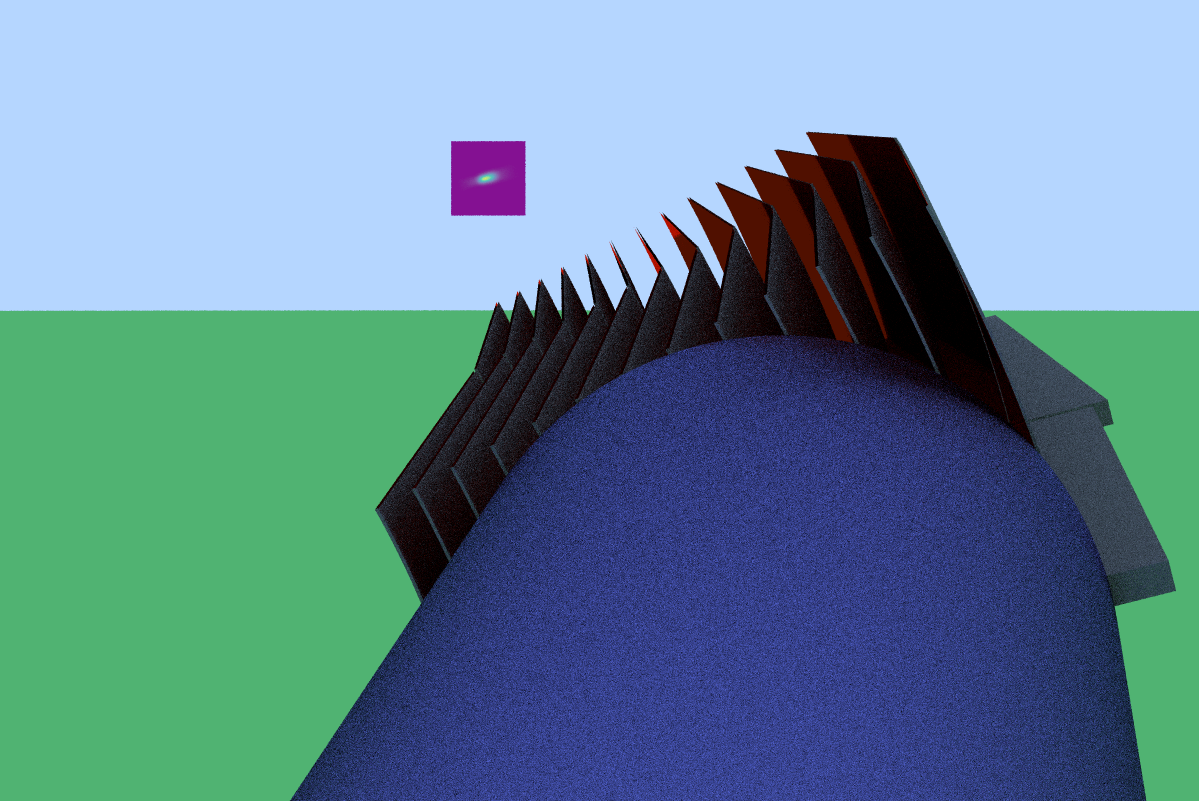
ImageSensor from on top of the magnet bore. The axion image is built up on the sensor and we view it "from above".Let's be more specific now about what these things mean precisely and how to get to the correct coordinate system we care about (looking 'at' the detector), taking into account the 90° rotation of the septemboard at CAST. Our target is the 'looking at' coordinates that fall out of TrAXer as seen in the screenshot. Let's use the term 'world coordinates' for this view.
- Description of our data reconstruction
As mentioned, our data reconstruction performs an inversion of the data seen 'from above' to 'through detector from behind'.
This means we perform a reflection along the \(y\) axis and perform a translation of 256 pixels, \(\vec{v}_x\)
A coordinate \((x, y)\) in the transformed coordinates becomes \((x', y')\), given by
\begin{align*} \vektor{x' \\ y'} &= \mathbf{T}_y · \vektor{x \\ y} + \vec{v}_x \\ &= \mtrix{ -1 & 0 \\ 0 & 1 } · \vektor{x \\ y} + \vektor{256 \\ 0} \\ &= \vektor{-x \\ y} + \vektor{256 \\ 0} \\ &= \vektor{256 - x \\ y} \\ &= \vektor{\tilde{x} \\ y} \end{align*}where we introduced \(\tilde{x}\) for our new inverted x-coordinates, given in millimeter.
(Note: we could make the translation more robust by using a 3D matrix (for this case) in homogeneous coordinates of the form
\[ \mathbf{V} = \mtrix{ 1 & 0 & 256 \\ 0 & 1 & 0 \\ 0 & 0 & 1 } \] where the last column performs a translation for us. Our input vectors would need to be extended by a third row, which we would set to 1. After applying the transformation we would then drop the 3rd dimension again. The result is essentially the same as above, but can be represented as a matrix product. This is commonly used in computer graphics { with there adding a 4th dimension to 3D vectors } )
- Description of the native data transformation
To convert the raw GridPix data (without the above inversion) into our target coordinates (in world coordinates) we need to account for the rotation of the GridPix detector. As described in the previous section, the detector is rotated by 90° clockwise (in world coordinates).
Rotations in mathematics commonly describe positive rotations as anti clockwise. Thus, our detector is rotated by \(\SI{-90}{°}\). Applying this rotation to our data yields the image as seen from world coordinates, mapped to the TrAXer simulation:
\begin{align*} \vektor{x' \\ y'} &= R_{\SI{-90}{°}} · \vektor{x \\ y} \\ &= \mtrix{ \cos θ & -\sin θ \\ \sin θ & \cos θ } · \vektor{x \\ y} \\ &= \mtrix{ 0 & 1 \\ -1 & 0 } · \vektor{x \\ y} \\ &= \vektor{y \\ -x} \end{align*}where we used \(θ = -π/2\).
- Comparing our current description to the target
Our current reconstructed data is of the form \((-x, y)\) while our target is \((y, -x)\). This means to get to the desired outcome all we have to do is replace the x and y coordinates. In other words perform a reflection along the line \(x = y\) in our data.
\begin{align*} \vektor{x' \\ y'} &= \mathbf{S}_{x = y} · \vektor{256 - x \\ y} \\ &= \mtrix{ 0 & 1 \\ 1 & 0 } · \vektor{256 - x \\ y} \\ &= \vektor{y \\ 256 - x} \end{align*}which is exactly what we want outside of the translation by \(\num{256}\), which is not strictly speaking there in our actual data, due to the data being converted into millimeter. But this just means the numbers are different, but the features are in the right place. That latter part is important. In our coordinated (inverted) data, the final transformation may look like \((y, \tilde{x})\) – clearly different from our target \((y, -x)\) – the underlying transformation is anyway of the form \((y, -x)\), barring a translation. That translation is essentially just dropped due to the millimeter conversion, but the inherent effect on the final geometry is anyway retained (and encoded in the fact that all x coordinates are reversed).
This means to bring our center cluster data to the same coordinates that we get from TrAXer (the world coordinates, 'looking at' the detector), all we need to do is to transpose our coordinates; replace x by y and vice versa.
From here we can cross check with the X-ray finger run, run 189, see fig. #fig:cast:xray_finger_centers generated in sec. 10.2.2, that this indeed makes sense. To quickly reproduce that figure here and compare it to our TrAXer raytracing for an X-ray finger run, see fig. 44.


In the plotting code in that section we implement the required transformation by exchanging the X by the Y center data. This is correct, but only because the conversion from pixel coordinates to milli meters when computing the cluster centers already includes the inversion of the x axis. A transposition like that should yield a clock wise rotation.
This means for our limit calculation: perform the same X ⇔ Y
replacement to get the correct rotation. Furthermore, let's look at an
X-ray finger run using TrAXer (read appendix
37 first) to reproduce the X-ray finger run of
run 189.
Note: the TrAXer raytracing binary output files that store the image sensor data are again inverted in y compared to what we see / what we want. In our detector the bottom left is \((0, 0)\). But the data buffer associated with an
ImageSensorin TrAXer starts with \((0, 0)\) in the top left. Hence you see--invertYin all calls toplotBinary!
13.15. Observed limit - \(g_{ae}\)
With the data fully unblinded and the solar tracking candidates known, we can now compute the observed limit for the axion-electron coupling \(g_{ae}\). We compute an observed limit of
\[ \left(g_{ae} · g_{aγ}\right)_{\text{observed}} = \SI{7.34(9)e-23}{GeV⁻¹}, \]
which is lower than the expected limit, due to the distribution of candidates and absence of any highly significant candidates. This limit is the mean value out of \(\num{200}\) limits computed via 3 Markov Chains of \(\num{150000}\) links (same as for the expected limits) computed for the real candidates. The printed uncertainty represents the standard deviation out of those limits. Therefore, we may wish to present an upper bound,
\[ \left(g_{ae} · g_{aγ}\right)_{\text{observed}} \lesssim \SI{7.35e-23}{GeV⁻¹} \text{ at } \SI{95}{\%} \text{ CL}. \]
The expected limit for this case was \(\left(g_{ae} · g_{aγ}\right)_{\text{expected}} = \SI{7.878225(6464)e-23}{GeV⁻¹}\) and the limit without any candidates at all \(\left(g_{ae} · g_{aγ}\right)_{\text{no candidates}} = \SI{6.39e-23}{GeV⁻¹}\).
This is a good improvement compared to the current, best observed limit by CAST in 2013 (Barth et al. 2013), which achieved
\[ \left(g_{ae} · g_{aγ}\right)_{\text{CAST2013}} \lesssim \SI{8.1e-23}{GeV⁻¹}. \]
Unfortunately, (Barth et al. 2013) does not provide an expected limit to compare to. 16
Fig. 45 shows the marginal posterior likelihood function for the observed solar tracking candidates, for a single calculation run (out of the \(\num{200}\) mentioned). The limit is at the \(95^{\text{th}}\) percentile of the histogram, shown by the intersection of the blue and red filling. In addition the yellow line shows values based on a numerical integration using Romberg's method (Romberg 1955) at 20 different coupling constants. This is a cross validation of the MCMC result. 17
Note that this observed limit is valid for axion masses in the range where the coherence condition in the conversion probability is met. That is, \(qL \ll π\), refer back to equation \eqref{eq:theory:axion_interaction:conversion_probability}. This holds up to axion masses around \(m_a \lesssim \SI{0.02}{eV}\), but the exact value is both energy dependent and based on the desired cutoff in reduction of the conversion probability. See fig. 195 in appendix 33.1 to see how the conversion probability develops as a function of axion mass. The expected and observed limits simply (inversely) follow the conversion probability, i.e. out of coherence they get exponentially worse, superimposed with the periodic modulation seen in the conversion probability. As we did not perform a buffer gas run, the behavior in that range is not computed, because it is mostly trivial (only the exact point at which the limit decreases changes depending on the exact energies of the candidates).
Finally, note that if one combines the existing astrophysical limits on \(g_{ae}\) alone (for example tip of the red giant branch star brightness limits, (Capozzi and Raffelt 2020) at \(g_{ae} < \num{1.3e-13}\)) with an axion-photon coupling of choice (for example the current best limit of (Collaboration and others 2017)) one may very well obtain a 'better' limit on \(g_{ae}·g_{aγ}\). In that sense the above, at the very least, represents the best helioscope limit on the product of both coupling constants. It also suffers less from uncertainties as astrophysical limits, see for example (Dennis and Sakstein 2023).

13.15.0.1. Sanity check extended
This is only one of them, but quick, gives an overview:
Running the sanity checks for the limits by varying g²_ae as
described in the thesis:
  mcmc_limit_calculation \
    sanity --limitKind lkMCMC \
    --axionModel ~/phd/resources/readOpacityFile/solar_axion_flux_differential_g_ae_1e-13_g_ag_1e-12_g_aN_1e-15_fluxKind_fkAxionElectronPhoton_0.989AU.csv \
    --axionImage ~/phd/resources/axionImages/solar_axion_image_fkAxionElectronPhoton_0.989AU_1492.93mm.csv \
    --combinedEfficiencyFile ~/org/resources/combined_detector_efficiencies.csv \
    --switchAxes --sanityPath ~/phd/Figs/limit/sanity/axionElectronSanity/ \
    --axionElectronLimit
See the plots in ./Figs/limit/sanity/axionElectronSanity/ and the sanity log:
  [2024-01-11 - 15:39:15] - INFO: =============== Input ===============
[2024-01-11 - 15:39:15] - INFO: 	Input path:
[2024-01-11 - 15:39:15] - INFO: 	Input files: @[(2017, "/home/basti/org/resources/lhood_mlp_17_11_23_adam_tanh30_sigmoid_mse_82k/lhood_c18_R2_crAll_sEff_0.95_scinti_fadc_line_mlp_mlp_tanh_sigmoid_MSE_Adam_30_2checkpoint_epoch_82000_loss_0.0249_acc_0.9662_vQ_0.99.h5"), (2018, "/home/basti/org/resources/lhood_mlp_17_11_23_adam_tanh30_sigmoid_mse_82k/lhood_c18_R3_crAll_sEff_0.95_scinti_fadc_line_mlp_mlp_tanh_sigmoid_MSE_Adam_30_2checkpoint_epoch_82000_loss_0.0249_acc_0.9662_vQ_0.99.h5")]
[2024-01-11 - 15:39:15] - INFO: =============== Time ===============
[2024-01-11 - 15:39:15] - INFO: 	Total background time: 3158.01 h
[2024-01-11 - 15:39:15] - INFO: 	Total tracking time: 159.899 h
[2024-01-11 - 15:39:15] - INFO: 	Ratio of tracking to background time: 1 UnitLess
[2024-01-11 - 15:39:16] - INFO: 	Saving plot: /home/basti/phd/Figs/limit/sanity/axionElectronSanity/candidates_signal_over_background_axion_electron.pdf
[2024-01-11 - 15:39:16] - INFO: =============== Chameleon coupling constant ===============
[2024-01-11 - 15:39:16] - INFO: 	Conversion probability using default g_aγ² = 9.999999999999999e-25, yields P_a↦γ = 1.62702e-21 UnitLess
[2024-01-11 - 15:39:25] - INFO: Limit with default g_ae² = 1e-26 is = 4.773876062173374e-21, and as g_ae = 6.909324179811926e-11
[2024-01-11 - 15:39:25] - INFO: 	Saving plot: /home/basti/phd/Figs/limit/sanity/axionElectronSanity/candidates_signal_over_background_axion_electron.pdf
[2024-01-11 - 15:39:37] - INFO: 2. Limit with default g_ae² = 1e-26 is = 8.300544615154112e-21, and as g_ae = 9.110732470638194e-11
[2024-01-11 - 15:39:37] - INFO: 	Saving plot: /home/basti/phd/Figs/limit/sanity/axionElectronSanity/candidates_signal_over_background_axion_electron.pdf
[2024-01-11 - 15:39:46] - INFO: 3. Limit with default g_ae² = 1e-26 is = 5.284512161896287e-21, and as g_ae = 7.26946501600791e-11
[2024-01-11 - 15:39:47] - INFO: 	Saving plot: /home/basti/phd/Figs/limit/sanity/axionElectronSanity/candidates_signal_over_background_axion_electron.pdf
[2024-01-11 - 15:39:58] - INFO: 4. Limit with default g_ae² = 1e-26 is = 5.92914993487365e-21, and as g_ae = 7.700097359692051e-11
And by varying g²ae·g²aγ instead (equivalent):
  mcmc_limit_calculation \
    sanity --limitKind lkMCMC \
    --axionModel ~/phd/resources/readOpacityFile/solar_axion_flux_differential_g_ae_1e-13_g_ag_1e-12_g_aN_1e-15_fluxKind_fkAxionElectronPhoton_0.989AU.csv \
    --axionImage ~/phd/resources/axionImages/solar_axion_image_fkAxionElectronPhoton_0.989AU_1492.93mm.csv \
    --combinedEfficiencyFile ~/org/resources/combined_detector_efficiencies.csv \
    --switchAxes --sanityPath ~/phd/Figs/limit/sanity/axionElectronAxionPhotonSanity/ \
    --axionElectronAxionPhotonLimit
see ./Figs/limit/sanity/axionElectronAxionPhotonSanity/ and the sanity log:
  [2024-01-11 - 15:42:04] - INFO: =============== Input ===============
[2024-01-11 - 15:42:04] - INFO: 	Input path:
[2024-01-11 - 15:42:04] - INFO: 	Input files: @[(2017, "/home/basti/org/resources/lhood_mlp_17_11_23_adam_tanh30_sigmoid_mse_82k/lhood_c18_R2_crAll_sEff_0.95_scinti_fadc_line_mlp_mlp_tanh_sigmoid_MSE_Adam_30_2checkpoint_epoch_82000_loss_0.0249_acc_0.9662_vQ_0.99.h5"), (2018, "/home/basti/org/resources/lhood_mlp_17_11_23_adam_tanh30_sigmoid_mse_82k/lhood_c18_R3_crAll_sEff_0.95_scinti_fadc_line_mlp_mlp_tanh_sigmoid_MSE_Adam_30_2checkpoint_epoch_82000_loss_0.0249_acc_0.9662_vQ_0.99.h5")]
[2024-01-11 - 15:42:05] - INFO: =============== Time ===============
[2024-01-11 - 15:42:05] - INFO: 	Total background time: 3158.01 h
[2024-01-11 - 15:42:05] - INFO: 	Total tracking time: 159.899 h
[2024-01-11 - 15:42:05] - INFO: 	Ratio of tracking to background time: 1 UnitLess
[2024-01-11 - 15:42:05] - INFO: 	Saving plot: /home/basti/phd/Figs/limit/sanity/axionElectronAxionPhotonSanity/candidates_signal_over_background_axion_electron_axion_photon.pdf
[2024-01-11 - 15:42:05] - INFO: =============== Axion-electron axion-photon coupling constant ===============
[2024-01-11 - 15:42:05] - INFO: 	Conversion probability using default g_aγ² = 9.999999999999999e-25, yields P_a↦γ = 1.62702e-21 UnitLess
[2024-01-11 - 15:42:14] - INFO: Limit is g_ae²·g_aγ² = 4.722738218023592e-45, as g_ae·g_aγ = 6.872218141199821e-23
[2024-01-11 - 15:42:14] - INFO: 	Saving plot: /home/basti/phd/Figs/limit/sanity/axionElectronAxionPhotonSanity/candidates_signal_over_background_axion_electron_axion_photon.pdf
[2024-01-11 - 15:42:25] - INFO: 2. Limit is g_ae²·g_aγ² = 8.597830720112351e-45, as g_ae·g_aγ = 9.272448824400355e-23
[2024-01-11 - 15:42:25] - INFO: 	Saving plot: /home/basti/phd/Figs/limit/sanity/axionElectronAxionPhotonSanity/candidates_signal_over_background_axion_electron_axion_photon.pdf
[2024-01-11 - 15:42:35] - INFO: 3. Limit is g_ae²·g_aγ² = 5.266187342850787e-45, as g_ae·g_aγ = 7.256850103764572e-23
[2024-01-11 - 15:42:35] - INFO: 	Saving plot: /home/basti/phd/Figs/limit/sanity/axionElectronAxionPhotonSanity/candidates_signal_over_background_axion_electron_axion_photon.pdf
[2024-01-11 - 15:42:46] - INFO: 4. Limit is g_ae²·g_aγ² = 6.027243097935441e-45, as g_ae·g_aγ = 7.763532120069731e-23
Compare the limits with the above to see that they are basically the same limits (the variation is down to the MCMC uncertainty for a single limit).
NOTE: Running the limit using --axionElectronAxionPhotonLimitWrong
will run it by varying g_ae·g_aγ (without the square) directly. This
is to illustrate the explanation of
sec. 13.12.2. It will show
a distorted histogram and different limits than in the above two
cases:
  mcmc_limit_calculation \
    sanity --limitKind lkMCMC \
    --axionModel ~/phd/resources/readOpacityFile/solar_axion_flux_differential_g_ae_1e-13_g_ag_1e-12_g_aN_1e-15_fluxKind_fkAxionElectronPhoton_0.989AU.csv \
    --axionImage ~/phd/resources/axionImages/solar_axion_image_fkAxionElectronPhoton_0.989AU_1492.93mm.csv \
    --combinedEfficiencyFile ~/org/resources/combined_detector_efficiencies.csv \
    --switchAxes --sanityPath ~/phd/Figs/limit/sanity/axionElectronAxionPhotonWrongSanity/ \
    --axionElectronAxionPhotonLimitWrong
See ./Figs/limit/sanity/axionElectronAxionPhotonWrongSanity/ and the sanity log:
  [2024-01-11 - 15:43:43] - INFO: =============== Input ===============
[2024-01-11 - 15:43:43] - INFO: 	Input path:
[2024-01-11 - 15:43:43] - INFO: 	Input files: @[(2017, "/home/basti/org/resources/lhood_mlp_17_11_23_adam_tanh30_sigmoid_mse_82k/lhood_c18_R2_crAll_sEff_0.95_scinti_fadc_line_mlp_mlp_tanh_sigmoid_MSE_Adam_30_2checkpoint_epoch_82000_loss_0.0249_acc_0.9662_vQ_0.99.h5"), (2018, "/home/basti/org/resources/lhood_mlp_17_11_23_adam_tanh30_sigmoid_mse_82k/lhood_c18_R3_crAll_sEff_0.95_scinti_fadc_line_mlp_mlp_tanh_sigmoid_MSE_Adam_30_2checkpoint_epoch_82000_loss_0.0249_acc_0.9662_vQ_0.99.h5")]
[2024-01-11 - 15:43:43] - INFO: =============== Time ===============
[2024-01-11 - 15:43:43] - INFO: 	Total background time: 3158.01 h
[2024-01-11 - 15:43:43] - INFO: 	Total tracking time: 159.899 h
[2024-01-11 - 15:43:43] - INFO: 	Ratio of tracking to background time: 1 UnitLess
[2024-01-11 - 15:43:43] - INFO: 	Saving plot: /home/basti/phd/Figs/limit/sanity/axionElectronAxionPhotonWrongSanity/candidates_signal_over_background_axion_electron_axion_photon_wrong.pdf
[2024-01-11 - 15:43:44] - INFO: =============== Axion-electron axion-photon coupling constant via g_ae·g_aγ directly ===============
[2024-01-11 - 15:43:44] - INFO: 	Conversion probability using default g_aγ² = 9.999999999999999e-25, yields P_a↦γ = 1.62702e-21 UnitLess
[2024-01-11 - 15:43:53] - INFO: Limit is g_ae·g_aγ = 5.536231179166123e-23
[2024-01-11 - 15:43:54] - INFO: 	Saving plot: /home/basti/phd/Figs/limit/sanity/axionElectronAxionPhotonWrongSanity/candidates_signal_over_background_axion_electron_axion_photon_wrong.pdf
[2024-01-11 - 15:44:05] - INFO: 2. Limit is g_ae·g_aγ = 7.677750408651383e-23
[2024-01-11 - 15:44:05] - INFO: 	Saving plot: /home/basti/phd/Figs/limit/sanity/axionElectronAxionPhotonWrongSanity/candidates_signal_over_background_axion_electron_axion_photon_wrong.pdf
[2024-01-11 - 15:44:15] - INFO: 3. Limit is g_ae·g_aγ = 5.828448006406443e-23
[2024-01-11 - 15:44:15] - INFO: 	Saving plot: /home/basti/phd/Figs/limit/sanity/axionElectronAxionPhotonWrongSanity/candidates_signal_over_background_axion_electron_axion_photon_wrong.pdf
[2024-01-11 - 15:44:27] - INFO: 4. Limit is g_ae·g_aγ = 6.573837668159744e-23
See how the limits are much lower than for the two cases above (the
additional 1e-12 difference is down to g_aγ not being included, note
the numbers outside of the power).
And in particular, compare

with the correct
 and
and

which illustrates the sampling behavior nicely.
13.15.0.2. Calculate the observed limit extended
We use F_WIDTH=0.5 for the ln(1 + s/b) plot. The MCMC gae²
histogram is forced to be 0.9 in width anyway.
    F_WIDTH=0.5 ESCAPE_LATEX=true USE_TEX=true mcmc_limit_calculation \
    limit \
    -f /home/basti/org/resources/lhood_mlp_17_11_23_adam_tanh30_sigmoid_mse_82k/lhood_c18_R2_crAll_sEff_0.95_scinti_fadc_line_mlp_mlp_tanh_sigmoid_MSE_Adam_30_2checkpoint_epoch_82000_loss_0.0249_acc_0.9662_vQ_0.99.h5 \
    -f /home/basti/org/resources/lhood_mlp_17_11_23_adam_tanh30_sigmoid_mse_82k/lhood_c18_R3_crAll_sEff_0.95_scinti_fadc_line_mlp_mlp_tanh_sigmoid_MSE_Adam_30_2checkpoint_epoch_82000_loss_0.0249_acc_0.9662_vQ_0.99.h5 \
    --tracking ~/org/resources/lhood_mlp_17_11_23_adam_tanh30_sigmoid_mse_82k_tracking/lhood_c18_R2_crAll_sEff_0.95_scinti_fadc_line_mlp_mlp_tanh_sigmoid_MSE_Adam_30_2checkpoint_epoch_82000_loss_0.0249_acc_0.9662_vQ_0.99.h5 \
    --tracking ~/org/resources/lhood_mlp_17_11_23_adam_tanh30_sigmoid_mse_82k_tracking/lhood_c18_R3_crAll_sEff_0.95_scinti_fadc_line_mlp_mlp_tanh_sigmoid_MSE_Adam_30_2checkpoint_epoch_82000_loss_0.0249_acc_0.9662_vQ_0.99.h5 \
    --axionModel ~/org/resources/axionProduction/axionElectronRealDistance/solar_axion_flux_differential_g_ae_1e-13_g_ag_1e-12_g_aN_1e-15_0.989AU.csv \
    --axionImage ~/phd/resources/axionImages/solar_axion_image_fkAxionElectronPhoton_0.989AU_1492.93mm.csv \
    --combinedEfficiencyFile ~/org/resources/combined_detector_efficiencies.csv \
    --switchAxes \
    --path "" \
    --years 2017 --years 2018 \
    --σ_p 0.05 \
    --energyMin 0.2 --energyMax 12.0 \
    --limitKind lkMCMC \
    --outpath ~/phd/Figs/trackingCandidates/ \
    --suffix ""
-> The plot looks exactly like the one already in the thesis? Surely they should be switched around x/y?
The log file: ./Figs/trackingCandidates/real_candidates_limit.log
13.16. Other coupling constants
As explained when we introduced the limit calculation method, one important aim was to develop a method which is agnostic to the coupling constant of choice. We will now make use of this to compute expected and observed limits for the axion-photon coupling \(g_{aγ}\), sec. 13.16.1 and chameleon coupling \(β_γ\), sec. 13.16.2.
13.16.1. Axion-photon coupling - \(g⁴_{aγ}\)
The axion-photon coupling requires the following changes:
- use \(g⁴_{aγ}\) in the vector of the Markov Chain, replacing the \(g²_{ae}\) term. As \(g_{aγ}\) both affects the production and reconversion it needs to be in the fourth power.
- the axion flux based on Primakoff production only.
- the axion image based on the Primakoff flux only.
The axion flux and axion image for the Primakoff production are shown in fig. 47. Note that the axion image is computed at the same effective conversion position as for the axion-electron flux. Strictly speaking this is not quite correct, due to the different energies of the two fluxes and therefore different absorption lengths. For the purposes here the inaccuracy is acceptable.
Based on these we compute an expected limit for the same setup that yielded the best expected limit for the axion-electron coupling constant. Namely, the MLP classifier at \(\SI{95}{\%}\) efficiency using all vetoes except the septem veto. We compute an expected limit based on \(\num{1e4}\) toy candidates. Fig. 48 shows the distribution of limits obtained for different toy candidates, including the expected limit. In appendix 33.2, tab. 35 the different percentiles for this distribution are shown. The obtained expected limit is
\[ g_{aγ, \text{expected}} = \SI{9.0650(75)e-11}{GeV⁻¹}, \]
which compared to the observed CAST Nature (Collaboration and others 2017) limit of \(g_{aγ, \text{Nature}} = \SI{6.6e-11}{GeV^{−1}}\) is of course significantly worse. This is expected however, due to significantly less tracking time and higher background rates. The limit without any candidates comes out to
\[ g_{aγ, \text{no candidates}} = \SI{7.95e-11}{GeV⁻¹}. \]
Based on the same candidates as in sec. 13.15 we obtain an observed limit of
\[ g_{aγ, \text{observed}} = \SI{8.99(7)e-11}{GeV⁻¹}, \]
which again is the mean out of 200 MCMC limits. Once again it is better than the expected limit, similar as for the axion-electron limit, but the overall result is as expected.
As a bound then, it is
\[ g_{aγ, \text{observed}} \lesssim \SI{9.0e-11}{GeV⁻¹} \text{ at } \SI{95}{\%} \text{ CL}. \]
The distribution of the posterior likelihood function can be found in fig. 196 of appendix 33.3.


13.16.1.1. Calculate differential axion-photon flux and emission rates extended
Same as for the axion-electron coupling, we use readOpacityFile with
the ~--fluxKind fkAxionPhoton argument (see also 37.4.3):
  ./readOpacityFile \
    --suffix "_0.989AU" \
    --distanceSunEarth 0.9891144450781392.AU \
    --fluxKind fkAxionPhoton \
    --plotPath ~/phd/Figs/readOpacityFile/ \
    --outpath ~/phd/resources/readOpacityFile/
13.16.1.2. Generate plot of differential Primakoff flux extended
Produce a standalone plot of the axion-photon flux:
    import ggplotnim, unchained
let df = readCsv(  "~/phd/resources/readOpacityFile/solar_axion_flux_differential_g_ae_1e-13_g_ag_1e-12_g_aN_1e-15_fluxKind_fkAxionPhoton_0.989AU.csv"  )
  .mutate(f{  float: "Flux" ~ idx(  "Flux / keV⁻¹ m⁻² yr⁻¹"  ).keV⁻¹•m⁻²•yr⁻¹.toDef(keV⁻¹•cm⁻²•s⁻¹).float  }  )
  .filter(f{  string: `type` == "Total flux"  }  )
ggplot(df, aes(  "Energy [keV]", "Flux"  )  ) +
  geom_line() +
  ylab(r"Flux [$\si{keV⁻¹.cm⁻².s⁻¹}$]"  ) +
  margin(left = 4.5  ) +
  ggtitle(r"Primakoff flux at $g_{aγ} = \SI{1e-12}{GeV⁻¹}$"  ) +
  xlim(  0.0, 15.0  ) +
  themeLatex(fWidth = 0.5, width = 600, baseTheme = sideBySide) +
  ggsave(  "~/phd/Figs/axions/differential_axion_flux_primakoff.pdf"  )
13.16.1.3. Generate axion image for axion-photon emission extended
Now we just run the raytracer, using the correct position (1492.93 mm effective distance from telescope center) and produced emission file:
  ./raytracer \
    --width 1200 --speed 10.0 --nJobs 32 --vfov 15 --maxDepth 5 \
    --llnl --focalPoint --sourceKind skSun \
    --solarModelFile ~/phd/resources/readOpacityFile/solar_model_dataframe_fluxKind_fkAxionPhoton_0.989AU.csv \
    --sensorKind sSum \
    --usePerfectMirror=false \
    --rayAt 0.995286666667 \
    --ignoreWindow
[INFO] Writing buffers to binary files. [INFO] Writing file: out/buffer2024-01-08T13:19:16+01:00typeuint32len1440000width1200height1200.dat [INFO] Writing file: out/counts2024-01-08T13:19:16+01:00typeintlen1440000width1200height1200.dat [INFO] Writing file: out/imagesensor02024-01-08T13:19:16+01:00_dx14.0dy14.0dz0.1typefloatlen1000000width1000height1000.dat
And plot it, produce the CSV axion image for the limit:
    F_WIDTH=0.5 USE_TEX=true ./plotBinary \
    --dtype float \
    -f out/image_sensor_0_2024-01-08T13:19:16+01:00__dx_14.0_dy_14.0_dz_0.1_type_float_len_1000000_width_1000_height_1000.dat \
    --invertY \
    --out ~/phd/Figs/raytracing/solar_axion_image_fkAxionPhoton_0.989AU_1492.93mm.pdf \
    --inPixels=false \
    --gridpixOutfile ~/phd/resources/axionImages/solar_axion_image_fkAxionPhoton_0.989AU_1492.93mm.csv \
    --title "Solar axion image (g_aγ) at 0.989 AU from Sun, 1492.93 mm"
yields:


13.16.1.4. Compute an expected limit extended
Given that this is only an 'add-on', we will just compute O(10k) toy limits for an expected limit using the best performing setup from the axion-electron limit. Based on those we will then compute the observed limit too.
Sanity checks:
  mcmc_limit_calculation \
    sanity --limitKind lkMCMC \
    --axionModel ~/phd/resources/readOpacityFile/solar_axion_flux_differential_g_ae_1e-13_g_ag_1e-12_g_aN_1e-15_fluxKind_fkAxionPhoton_0.989AU.csv \
    --axionImage ~/phd/resources/axionImages/solar_axion_image_fkAxionPhoton_0.989AU_1492.93mm.csv \
    --combinedEfficiencyFile ~/org/resources/combined_detector_efficiencies.csv \
    --switchAxes --sanityPath ~/phd/Figs/limit/sanity/axionPhotonSanity/ \
    --axionPhotonLimit
see ./Figs/limit/sanity/axionPhotonSanity/ and the sanity log file:
  [2024-01-11 - 15:48:04] - INFO: =============== Input ===============
[2024-01-11 - 15:48:04] - INFO: 	Input path:
[2024-01-11 - 15:48:04] - INFO: 	Input files: @[(2017, "/home/basti/org/resources/lhood_mlp_17_11_23_adam_tanh30_sigmoid_mse_82k/lhood_c18_R2_crAll_sEff_0.95_scinti_fadc_line_mlp_mlp_tanh_sigmoid_MSE_Adam_30_2checkpoint_epoch_82000_loss_0.0249_acc_0.9662_vQ_0.99.h5"), (2018, "/home/basti/org/resources/lhood_mlp_17_11_23_adam_tanh30_sigmoid_mse_82k/lhood_c18_R3_crAll_sEff_0.95_scinti_fadc_line_mlp_mlp_tanh_sigmoid_MSE_Adam_30_2checkpoint_epoch_82000_loss_0.0249_acc_0.9662_vQ_0.99.h5")]
[2024-01-11 - 15:48:05] - INFO: =============== Time ===============
[2024-01-11 - 15:48:05] - INFO: 	Total background time: 3158.01 h
[2024-01-11 - 15:48:05] - INFO: 	Total tracking time: 159.899 h
[2024-01-11 - 15:48:05] - INFO: 	Ratio of tracking to background time: 1 UnitLess
[2024-01-11 - 15:48:05] - INFO: 	Saving plot: /home/basti/phd/Figs/limit/sanity/axionPhotonSanity/candidates_signal_over_background_axionPhoton.pdf
[2024-01-11 - 15:48:05] - INFO: =============== Axion-photon coupling constant ===============
[2024-01-11 - 15:48:05] - INFO: 	Conversion probability using default g_aγ² = 9.999999999999999e-25, yields P_a↦γ = 7.97241e-18 UnitLess
[2024-01-11 - 15:48:24] - INFO: Limit with default g_aγ² = 9.999999999999999e-25 is = 5.348452506385883e-41, and as g_aγ = 8.551790162182624e-11
[2024-01-11 - 15:48:24] - INFO: 	Saving plot: /home/basti/phd/Figs/limit/sanity/axionPhotonSanity/candidates_signal_over_background_axionPhoton.pdf
[2024-01-11 - 15:48:45] - INFO: 2. Limit with default g_aγ² = 9.999999999999999e-25 is = 9.258158870434389e-41, and as g_aγ = 9.809145065039609e-11
[2024-01-11 - 15:48:45] - INFO: 	Saving plot: /home/basti/phd/Figs/limit/sanity/axionPhotonSanity/candidates_signal_over_background_axionPhoton.pdf
[2024-01-11 - 15:49:04] - INFO: 3. Limit with default g_aγ² = 9.999999999999999e-25 is = 6.93624112433336e-41, and as g_aγ = 9.126012210624729e-11
[2024-01-11 - 15:49:04] - INFO: 	Saving plot: /home/basti/phd/Figs/limit/sanity/axionPhotonSanity/candidates_signal_over_background_axionPhoton.pdf
[2024-01-11 - 15:49:25] - INFO: 4. Limit with default g_aγ² = 9.999999999999999e-25 is = 6.105369380817466e-41, and as g_aγ = 8.839505819701355e-11
The limits seem reasonable for our detector. Worse than the Nature limit by quite a bit, but still acceptable!
See sec. 13.13.5 for the command for axion-electron using 50k toys. The main differences:
- axion photon differential flux
- axion photon axion image
- couplingKind: gaγ
  mcmc_limit_calculation \
    limit \
    -f /home/basti/org/resources/lhood_mlp_17_11_23_adam_tanh30_sigmoid_mse_82k/lhood_c18_R2_crAll_sEff_0.95_scinti_fadc_line_mlp_mlp_tanh_sigmoid_MSE_Adam_30_2checkpoint_epoch_82000_loss_0.0249_acc_0.9662_vQ_0.99.h5 \
    -f /home/basti/org/resources/lhood_mlp_17_11_23_adam_tanh30_sigmoid_mse_82k/lhood_c18_R3_crAll_sEff_0.95_scinti_fadc_line_mlp_mlp_tanh_sigmoid_MSE_Adam_30_2checkpoint_epoch_82000_loss_0.0249_acc_0.9662_vQ_0.99.h5 \
    --axionModel ~/phd/resources/readOpacityFile/solar_axion_flux_differential_g_ae_1e-13_g_ag_1e-12_g_aN_1e-15_fluxKind_fkAxionPhoton_0.989AU.csv \
    --axionImage ~/phd/resources/axionImages/solar_axion_image_fkAxionPhoton_0.989AU_1492.93mm.csv \
    --combinedEfficiencyFile ~/org/resources/combined_detector_efficiencies.csv \
    --switchAxes \
    --path "" \
    --years 2017 --years 2018 \
    --σ_p 0.05 \
    --energyMin 0.2 --energyMax 12.0 \
    --limitKind lkMCMC \
    --couplingKind ck_g_aγ⁴ \
    --outpath ~/org/resources/lhood_limits_axion_photon_11_01_24/lhood_c18_R2_crAll_sEff_0.95_scinti_fadc_septem_line_mlp_mlp_tanh_sigmoid_MSE_Adam_30_2checkpoint_epoch_82000_loss_0.0249_acc_0.9662_vQ_0.99/ \
    --suffix "" \
    --nmc 10000
Expected limit: 6.752456878081697e-41 Generating group /ctx/trackingDf Generating group /ctx/axionModel Serializing Interpolator by evaluating 0.001 to 15.0 of name: axionSpl Serializing Interpolator by evaluating 0.0 to 10.0 of name: efficiencySpl Serializing Interpolator by evaluating 0.2 to 12.0 of name: backgroundSpl Generating group /ctx/backgroundDf Wrote outfile /home/basti/org/resources/lhoodlimitsaxionphoton110124/lhoodc18R2crAllsEff0.95scintifadcseptemlinemlpmlptanhsigmoidMSEAdam302checkpointepoch82000loss0.0249acc0.9662vQ0.99/mclimitlkMCMCskInterpBackgroundnmc10000uncertaintyukUncertainσs0.0276σb0.0028posUncertainpuUncertainσp0.0500.h5
Finished . It took about 3 hours maybe.
[ ]Make the output plot prettier! It's super ugly due to a few very large limits.
./generateExpectedLimitsTable --path ~/org/resources/lhood_limits_axion_photon_11_01_24/ --prefix "mc_limit_lkMCMC" --precision 2 --coupling ck_g_aγ⁴
13.16.1.5. Generate plot of expected limit histogram extended
    ESCAPE_LATEX=true USE_TEX=true mcmc_limit_calculation \
    limit \
    -f /home/basti/org/resources/lhood_mlp_17_11_23_adam_tanh30_sigmoid_mse_82k/lhood_c18_R2_crAll_sEff_0.95_scinti_fadc_line_mlp_mlp_tanh_sigmoid_MSE_Adam_30_2checkpoint_epoch_82000_loss_0.0249_acc_0.9662_vQ_0.99.h5 \
    -f /home/basti/org/resources/lhood_mlp_17_11_23_adam_tanh30_sigmoid_mse_82k/lhood_c18_R3_crAll_sEff_0.95_scinti_fadc_line_mlp_mlp_tanh_sigmoid_MSE_Adam_30_2checkpoint_epoch_82000_loss_0.0249_acc_0.9662_vQ_0.99.h5 \
    --axionModel ~/phd/resources/readOpacityFile/solar_axion_flux_differential_g_ae_1e-13_g_ag_1e-12_g_aN_1e-15_fluxKind_fkAxionPhoton_0.989AU.csv \
    --axionImage ~/phd/resources/axionImages/solar_axion_image_fkAxionPhoton_0.989AU_1492.93mm.csv \
    --combinedEfficiencyFile ~/org/resources/combined_detector_efficiencies.csv \
    --path "" \
    --years 2017 --years 2018 \
    --σ_p 0.05 \
    --energyMin 0.2 --energyMax 12.0 \
    --plotFile ~/org/resources/lhood_limits_axion_photon_11_01_24/lhood_c18_R2_crAll_sEff_0.95_scinti_fadc_septem_line_mlp_mlp_tanh_sigmoid_MSE_Adam_30_2checkpoint_epoch_82000_loss_0.0249_acc_0.9662_vQ_0.99/mc_limit_lkMCMC_skInterpBackground_nmc_10000_uncertainty_ukUncertain_σs_0.0276_σb_0.0028_posUncertain_puUncertain_σp_0.0500.csv \
    --xLow 2e-41 \
    --xHigh 2e-40 \
    --couplingKind ck_g_aγ⁴ \
    --limitKind lkMCMC \
    --yHigh 400 \
    --bins 100 \
    --linesTo 220 \
    --xLabel "Limit g_aγ⁴ [GeV⁻⁴]" \
    --yLabel "MC toy count"  \
    --outpath ~/phd/Figs/limit/ \
    --suffix "_axion_photon_nmc_10k_pretty" \
    --nmc 10000
13.16.1.6. Calculate the observed limit extended
We use F_WIDTH=0.5 for the ln(1 + s/b) plot. The MCMC gae²
histogram is forced to be 0.9 in width anyway.
    F_WIDTH=0.5 ESCAPE_LATEX=true USE_TEX=true mcmc_limit_calculation \
    limit \
    -f /home/basti/org/resources/lhood_mlp_17_11_23_adam_tanh30_sigmoid_mse_82k/lhood_c18_R2_crAll_sEff_0.95_scinti_fadc_line_mlp_mlp_tanh_sigmoid_MSE_Adam_30_2checkpoint_epoch_82000_loss_0.0249_acc_0.9662_vQ_0.99.h5 \
    -f /home/basti/org/resources/lhood_mlp_17_11_23_adam_tanh30_sigmoid_mse_82k/lhood_c18_R3_crAll_sEff_0.95_scinti_fadc_line_mlp_mlp_tanh_sigmoid_MSE_Adam_30_2checkpoint_epoch_82000_loss_0.0249_acc_0.9662_vQ_0.99.h5 \
    --tracking ~/org/resources/lhood_mlp_17_11_23_adam_tanh30_sigmoid_mse_82k_tracking/lhood_c18_R2_crAll_sEff_0.95_scinti_fadc_line_mlp_mlp_tanh_sigmoid_MSE_Adam_30_2checkpoint_epoch_82000_loss_0.0249_acc_0.9662_vQ_0.99.h5 \
    --tracking ~/org/resources/lhood_mlp_17_11_23_adam_tanh30_sigmoid_mse_82k_tracking/lhood_c18_R3_crAll_sEff_0.95_scinti_fadc_line_mlp_mlp_tanh_sigmoid_MSE_Adam_30_2checkpoint_epoch_82000_loss_0.0249_acc_0.9662_vQ_0.99.h5 \
    --axionModel ~/phd/resources/readOpacityFile/solar_axion_flux_differential_g_ae_1e-13_g_ag_1e-12_g_aN_1e-15_fluxKind_fkAxionPhoton_0.989AU.csv \
    --axionImage ~/phd/resources/axionImages/solar_axion_image_fkAxionPhoton_0.989AU_1492.93mm.csv \
    --combinedEfficiencyFile ~/org/resources/combined_detector_efficiencies.csv \
    --couplingKind ck_g_aγ⁴ \
    --switchAxes \
    --path "" \
    --years 2017 --years 2018 \
    --σ_p 0.05 \
    --energyMin 0.2 --energyMax 12.0 \
    --limitKind lkMCMC \
    --outpath ~/phd/Figs/trackingCandidates/axionPhoton/ \
    --suffix ""
The log file: ./Figs/trackingCandidates/axionPhoton/real_candidates_limit.log
  [2024-01-18 - 14:18:05] - INFO: Mean of 200 real limits (3·150k MCMC) = 8.999457e-11
[2024-01-18 - 14:18:05] - INFO: Median of 200 real limits (3·150k MCMC) = 8.991653e-11
[2024-01-18 - 14:18:05] - INFO: σ of 200 real limits (3·150k MCMC) = 7.388529e-13
[2024-01-18 - 14:18:05] - INFO: Combined real limit (200 times 3·150k MCMC) = 8.99946(7389)e-11
[2024-01-18 - 14:18:05] - INFO: Real limit based on 3 150k long MCMCs: g_aγ = 8.961844793705987e-11
(that should read gaγ⁴, to be updated), yields \(g_aγ = \SI{8.99946(7389)e-11}{GeV⁻¹}\)
13.16.2. Chameleon coupling - \(β⁴_γ\)
Let's now have a look at the chameleon coupling. In addition to the inputs and MCMC parameter that needs to be changed similarly to the axion-photon coupling (flux, image and using \(β^4_γ\) in the MCMC), the conversion probability needs to be adjusted according to eq. \eqref{eq:theory:chameleon_conversion_prob}. This assumes the conversion is fully coherent and we restrict ourselves to non-resonant production. That means a chameleon-matter coupling \(β_m\) of
\[ 1 \leq β_m \leq \num{1e6}. \]
Further, because the chameleon production occurs in the solar tachocline – at around \(0.7 · R_{\odot}\) – the angles under which chameleons can reach the CAST magnet are much larger than for axions. This leads to a significant fraction of chameleons not traversing the entire magnet. For any chameleon traversing only parts of it, its probability for conversion is decreased. According to (Anastassopoulos et al. 2015) this is accounted for by a correction factor of \(\SI{38.9}{\%}\) in reduction of signal. (Christoph Krieger 2018) used a simplified raytracing model for this. While the distance through the magnet can easily be modeled with our raytracer (see appendix 37), we will still use the correction factor 18.
Fig. 49 shows the differential chameleon flux, assuming a magnetic field of \(\SI{10}{T}\) at the solar tachocline region and using \(β_γ = β^{\text{sun}}_γ = \num{6.46e10}\) (the bound on the chameleon coupling from solar physics). The chameleon image is in stark contrast to the very small axion image seen in the previous sections. The outer most ring corresponds to production in the tachocline regions in which our view is effectively tangent to the tachocline normal (i.e. the 'outer ring' of the solar tachocline when looking at the Sun). Also visible is the asymmetry in the signal on the chip, due to the LLNL telescope. The densest flux regions are in the top and bottom. These correspond to the narrow sides of the ellipsoid for example in fig. 47(b). This 'focusing effect' was not visible in the raytracing simulation of (Christoph Krieger 2018), due to the simpler raytracing approach, which approximated the ABRIXAS telescope as a lens (slight differences between ABRIXAS and LLNL telescope would of course exist).
The relative size of the chameleon image compared to the size of the GridPix was one of the main motivators to implement the background interpolation as introduced in sec. 13.10.8. This allows us to utilize the entire chameleon flux and weigh each chameleon candidate correctly. This is a significant improvement compared to the 2014/15 detector result (Christoph Krieger 2018), in which the entire outer ring of the chameleon flux had to be dropped. Not only can we include these regions in our calculation due to our approach, but also our background level is significantly lower in these outer regions thanks to the usage of our vetoes (compare fig. #fig:background:background_suppression_comparison, where #fig:background:suppression_lnL80_without is comparable to the background level of (Christoph Krieger 2018)).
Again, we follow the approach used for the axion-photon coupling and restrict ourselves to a single calculation of an expected limit for the best veto setup (MLP at \(\SI{95}{\%}\) efficiency using vetoes except the septem veto) based on \(\num{1e4}\) toy candidate sets. This yields an expected limit of
\[ β_{γ, \text{expected}} = \num{3.6060(39)e+10}. \]
Without any candidates, which for the chameleon due to its large much larger focused image is significantly more extreme, the limit comes out to
\[ β_{γ, \text{no candidates}} = \num{2.62e10}. \]
Fig. 50 shows the histograms of these toy limits. The differently colored histograms are again based on an arbitrary cutoff in \(\ln(1 + s/b)\) for a fixed coupling constant. We can see that the difference between the 'no candidate' limit and the lowest toy limits is much larger than for the two axion limits. This is due to the chameleon image covering a large fraction of the chip, making it incredibly unlikely to have no candidates. Further, in appendix 33.2 we find tab. 36, containing the different percentiles for the distribution of toy limits.
For the chameleon coupling it may be worthwhile to investigate other veto setups again, because of the very different nature of the chameleon image and even lower peak of the differential flux. Based on the same setup we compute an observed limit using the same set of candidates as previously of
\[ β_{γ, \text{observed}} = \num{3.10(2)e+10}. \]
or as an upper bound
\[ β_{γ, \text{observed}} \lesssim \num{3.1e+10} \text{ at } \SI{95}{\%} \text{ CL}. \]
This is a good improvement over the limit of (Christoph Krieger 2018; Anastassopoulos et al. 2019), and the current best chameleon-photon bound, of
\[ β_{γ, \text{Krieger}} = \num{5.74e10} \text{ at } \SI{95}{\%} \text{ CL}. \]
despite significantly less solar tracking time than in the former (our \(\SI{160}{h}\) to \(\SI{254}{h}\) in (Christoph Krieger 2018)), thanks to the significant improvements in background due to the detector vetoes, higher detection efficiency (thinner window), better classifier and improved limit calculation method allowing for the inclusion of the entire chameleon flux.
A figure of the sampled coupling constants, similar to fig. 45 can be found in appendix 33.4, fig. 197.
Note however, that it is somewhat surprising that the observed limit is also an improvement over the expected limit, as the total number of clusters in the tracking data is almost exactly as expected (850 for 844 expected). Based on all evaluations I have done, it seems to be a real effect of the candidates. In fig. 38(b) of the spectrum comparing candidates to background, we see that there is a slight, but noticeable lower rate at energies below \(\SI{2}{keV}\), which is the relevant range for chameleons. As such it may very well be a real effect, despite putting it below the \(5^{\text{th}}\) percentile of the toy limits (compare tab. 36). Further investigation seems appropriate.


13.16.2.1. Chameleon references extended
For chameleon theory. Best overview in detail:
~/Documents/Papers/PapersHome/Masterarbeit/Chameleons/thoroughchameleonreview0611816.pdf
later review: chameleonreview1602.03869.pdf
To differentiate chameleon gravity from other GR extensions: especially ~/Documents/Papers/braxdistinguishingmodifiedgravitymodels1506.01519.pdf and ~/Documents/Papers/braxlecturesonscreenedmodifiedgravity1211.5237v1.pdf
Detection in experiments, e.g. CAST ~/Documents/Papers/braxdetectionchameleons1110.2583.pdf and a bit braxsolarchameleons1004.1846v1.pdf (is this a precursor preprint?)
Other reading: chameleons and solar physics: chameleonsandsolarphysics1405.1581.pdf
polarizationsproducedbychameleonsPhysRevD.79.044028.pdf
13.16.2.2. Chameleon spectrum and plot extended
We have the chameleon spectrum from Christoph's limit code back in the
day. The file ./resources/chameleon-spectrum.dat contains the flux
in units of 1/16mm2/hour/keV at β_m = β^sun_m = 10^10.81 assuming
a magnetic field of 10 T at the solar tachocline, iirc.
./../org/Misc/chameleon_spectrum.nim
[ ]Insert flux!
    import ggplotnim, unchained

#   The data file `  chameleon-spectrum.dat  ` contains the spectrum in units of
#   `  keV⁻¹•16mm⁻²•h⁻¹  ` at β_m = β_m^sun = 6.457e10 or 10^10.81.
#   See fig. 11.2 in Christoph's thesis
defUnit(keV⁻¹•mm⁻²•h⁻¹)
defUnit(keV⁻¹•cm⁻²•s⁻¹)
func conversionProbabilityChameleon  (  B: Tesla, L: Meter  ): float =
  const M_pl = sqrt(  (  (hp_bar * c) / G_Newton  ).toDef(kg²)  ).toNaturalUnit.to(  GeV  ) / sqrt(  8 * π) #   reduced Planck mass in natural units
  const βγsun = pow(  10, 10.81  )
  let M_γ = M_pl / βγsun
  result = (  B.toNaturalUnit * L.toNaturalUnit / (  2 * M_γ  )  )^2
proc convertChameleon  (x: float  ): float =
  #   divide by 16 to get from  /16mm² to /1mm². Input f
  #   idiotic flux has already taken conversion probability into account.
  let P = conversionProbabilityChameleon(  9.0.T, 9.26.m) #   used values by Christop!
  result = (x.keV⁻¹•mm⁻²•h⁻¹ / 16.0 / P  ).to(keV⁻¹•cm⁻²•s⁻¹).float

let df = readCsv(  "~/phd/resources/chameleon-spectrum.dat", sep = '\t', header = "#"  )
  .mutate(f{  "Flux" ~ convertChameleon(idx(  "I[/16mm2/hour/keV]"  )  )  },
          f{  "Energy [keV]" ~ `energy` / 1000.0  }  )
ggplot(df, aes(  "Energy [keV]", "Flux"  )  ) +
  geom_line() +
  ylab(r"Flux [$\si{keV⁻¹.cm⁻².s⁻¹}$]"  ) +
  margin(left = 4.5  ) +
  ggtitle(r"Chameleon flux at $β^{\text{sun}}_γ = \num{6.46e10}$"  ) +
  themeLatex(fWidth = 0.5, width = 600, baseTheme = sideBySide) +
  ggsave(  "~/phd/Figs/axions/differential_chameleon_flux.pdf"  )
13.16.2.3. Conversion probability extended
Chameleon references: (Anastassopoulos et al. 2019) (Anastassopoulos et al. 2015)
Conversion probability for back conversion. We are in the coherent regime. In this case (Brax, Lindner, and Zioutas 2012) equation 52:
\[ P_{c↦γ} = \frac{B² L²}{4 M²_γ} \]
where \(M_γ\) is defined implicitly via the chameleon-photon coupling \(β_γ\),
\[ β_γ = \frac{m_{\text{pl}}}{M_γ} \]
where \(m_{\text{pl}}\) is the reduced Planck mass, \(m_{\text{pl}} = \frac{M_{\text{pl}}}{\sqrt{8 π}}\) (i.e. using natural units with \(G = \frac{1}{8π}\) instead of \(G = 1\), used in cosmology because it removes the \(8π\) term from the Einstein field equations). See (Anastassopoulos et al. 2019) for mention that it is the reduced Planck constant here. But the \(\sim \SI{2e18}{GeV}\) also gives it away. Let's check that the numbers hold:
    import unchained

let M_pl = sqrt (  (hp_bar * c) / G_Newton  ).toDef(kg²)
echo "Planck mass = ", M_pl, " in GeV = ", M_pl.toNaturalUnit.to(  GeV  ) / sqrt(  8 * π)
which indeed matches (although 2 is a rough approximation of the value!).
Let's compute the conversion probability for a single \(β_γ\) value:
    import unchained

proc conversionProbability  (  B: Tesla, L: Meter, β_γ: float  ): float =
  let M_pl = sqrt(  (  (hp_bar * c) / G_Newton  ).toDef(kg²)  ).toNaturalUnit.to(  GeV  ) / sqrt(  8 * π)
  #  let M_γ = M_pl / β_γ
  result = (β_γ * B.toNaturalUnit() * L.toNaturalUnit() / (  2 * M_pl  )  )^2

echo "Conversion probability: ", conversionProbability(  8.8.T, 9.26.m, 5.6e10)
O(1e-12) seems somewhat reasonable, given that the flux is generally much lower than for axions? But maybe the flux is too low? The flux is on the order of 1e-4 keV⁻¹•cm⁻²•s⁻¹ after all.
Let's compare:
    import unchained, math
defUnit(cm²)
defUnit(keV⁻¹)

func conversionProbability  (): UnitLess =
  ## the conversion probability in the CAST magnet (depends on g_aγ)
  ## simplified vacuum conversion prob. for small masses
  let B = 9.0.T
  let L = 9.26.m
  let g_aγ = 1e-12.GeV⁻¹ #   ``  must  `` be same as reference in Context
  result = pow( (g_aγ * B.toNaturalUnit * L.toNaturalUnit / 2.0  ), 2.0 )
echo conversionProbability()
    import unchained

let flx = 2e18.keV⁻¹•m⁻²•yr⁻¹
echo flx.toDef(keV⁻¹•cm⁻²•s⁻¹)
So 6e6 axions at 1.7e-21 vs 8.6e-13 at 1e-4:
    echo 6e6 * 1.7e-21
echo 1e-4 * 8.6e-13
3 orders of magnitude difference. That seems like it would be too much? Surely not made up by the fact that the area of interest is so much larger, no? Only one way to find out, I guess.
13.16.2.4. Generate chameleon solar image extended
  ./raytracer \
    --width 1200 --speed 10.0 --nJobs 32 --vfov 15 --maxDepth 5 \
    --llnl --focalPoint --sourceKind skSun \
    --chameleonFile ~/org/resources/chameleon-spectrum.dat \
    --sensorKind sSum \
    --usePerfectMirror=false \
    --ignoreWindow \
    --ignoreMagnet
[INFO] Writing buffers to binary files. [INFO] Writing file: out/buffer2024-01-08T20:29:05+01:00typeuint32len1440000width1200height1200.dat [INFO] Writing file: out/counts2024-01-08T20:29:05+01:00typeintlen1440000width1200height1200.dat [INFO] Writing file: out/imagesensor02024-01-08T20:29:05+01:00_dx14.0dy14.0dz0.1typefloatlen1000000width1000height1000.dat
    F_WIDTH=0.5 USE_TEX=true ./plotBinary \
    --dtype float \
    -f out/image_sensor_0_2024-01-08T20:29:05+01:00__dx_14.0_dy_14.0_dz_0.1_type_float_len_1000000_width_1000_height_1000.dat \
    --invertY \
    --out ~/phd/Figs/raytracing/solar_chameleon_image_0.989AU_1500mm.pdf \
    --inPixels=false \
    --gridpixOutfile ~/phd/resources/axionImages/solar_chameleon_image_0.989AU_1500mm.csv \
    --title "Solar chameleon image at 0.989 AU from Sun, 1500 mm"
13.16.2.5. Compute an expected limit extended
Sanity checks:
  mcmc_limit_calculation \
    sanity --limitKind lkMCMC \
    --axionModel ~/phd/resources/chameleon-spectrum.dat \
    --isChameleon \
    --axionImage ~/phd/resources/axionImages/solar_chameleon_image_0.989AU_1500mm.csv \
    --combinedEfficiencyFile ~/org/resources/combined_detector_efficiencies.csv \
    --switchAxes --sanityPath ~/phd/Figs/limit/sanity/chameleonSanity \
    --chameleonLimit
see ./Figs/limit/sanity/chameleonSanity/ and the sanity log file:
  [2024-01-11 - 15:50:40] - INFO: =============== Input ===============
[2024-01-11 - 15:50:40] - INFO: 	Input path:
[2024-01-11 - 15:50:40] - INFO: 	Input files: @[(2017, "/home/basti/org/resources/lhood_mlp_17_11_23_adam_tanh30_sigmoid_mse_82k/lhood_c18_R2_crAll_sEff_0.95_scinti_fadc_line_mlp_mlp_tanh_sigmoid_MSE_Adam_30_2checkpoint_epoch_82000_loss_0.0249_acc_0.9662_vQ_0.99.h5"), (2018, "/home/basti/org/resources/lhood_mlp_17_11_23_adam_tanh30_sigmoid_mse_82k/lhood_c18_R3_crAll_sEff_0.95_scinti_fadc_line_mlp_mlp_tanh_sigmoid_MSE_Adam_30_2checkpoint_epoch_82000_loss_0.0249_acc_0.9662_vQ_0.99.h5")]
[2024-01-11 - 15:50:41] - INFO: =============== Time ===============
[2024-01-11 - 15:50:41] - INFO: 	Total background time: 3158.01 h
[2024-01-11 - 15:50:41] - INFO: 	Total tracking time: 159.899 h
[2024-01-11 - 15:50:41] - INFO: 	Ratio of tracking to background time: 1 UnitLess
[2024-01-11 - 15:50:41] - INFO: 	Saving plot: /home/basti/phd/Figs/limit/sanity/chameleonSanity/candidates_signal_over_background_chameleon.pdf
[2024-01-11 - 15:50:41] - INFO: =============== Chameleon coupling constant ===============
[2024-01-11 - 15:50:41] - INFO: 	Conversion probability using default β² = 4.168693834703363e+21, yields P_c↦γ = 1.06716e-14 UnitLess
[2024-01-11 - 15:50:52] - INFO: Limit with default β² = 4.168693834703363e+21 is = 1.637454027281386e+42, and as β = 3.577192e+10
[2024-01-11 - 15:50:52] - INFO: 	Saving plot: /home/basti/phd/Figs/limit/sanity/chameleonSanity/candidates_signal_over_background_chameleon.pdf
[2024-01-11 - 15:51:03] - INFO: 2. Limit with default β² = 4.168693834703363e+21 is = 2.129378077440907e+42, and as β = 3.819999e+10
[2024-01-11 - 15:51:04] - INFO: 	Saving plot: /home/basti/phd/Figs/limit/sanity/chameleonSanity/candidates_signal_over_background_chameleon.pdf
[2024-01-11 - 15:51:15] - INFO: 3. Limit with default β² = 4.168693834703363e+21 is = 1.890732758560203e+42, and as β = 3.708152e+10
[2024-01-11 - 15:51:15] - INFO: 	Saving plot: /home/basti/phd/Figs/limit/sanity/chameleonSanity/candidates_signal_over_background_chameleon.pdf
[2024-01-11 - 15:51:26] - INFO: 4. Limit with default β² = 4.168693834703363e+21 is = 1.391973234680927e+42, and as β = 3.434850e+10
These limits look good! Quite a bit better than Christoph's (which was 5.5e10).
See sec. 13.13.5 for the command for axion-electron using 50k toys. The main differences:
- chameleon differential flux
- chameleon axion image
- couplingKind: βm
  mcmc_limit_calculation \
    limit \
    -f /home/basti/org/resources/lhood_mlp_17_11_23_adam_tanh30_sigmoid_mse_82k/lhood_c18_R2_crAll_sEff_0.95_scinti_fadc_line_mlp_mlp_tanh_sigmoid_MSE_Adam_30_2checkpoint_epoch_82000_loss_0.0249_acc_0.9662_vQ_0.99.h5 \
    -f /home/basti/org/resources/lhood_mlp_17_11_23_adam_tanh30_sigmoid_mse_82k/lhood_c18_R3_crAll_sEff_0.95_scinti_fadc_line_mlp_mlp_tanh_sigmoid_MSE_Adam_30_2checkpoint_epoch_82000_loss_0.0249_acc_0.9662_vQ_0.99.h5 \
    --axionModel ~/phd/resources/chameleon-spectrum.dat \
    --isChameleon \
    --axionImage ~/phd/resources/axionImages/solar_chameleon_image_0.989AU_1500mm.csv \
    --combinedEfficiencyFile ~/org/resources/combined_detector_efficiencies.csv \
    --couplingKind ck_β⁴ \
    --switchAxes \
    --path "" \
    --years 2017 --years 2018 \
    --σ_p 0.05 \
    --energyMin 0.2 --energyMax 12.0 \
    --limitKind lkMCMC \
    --outpath ~/org/resources/lhood_limits_chameleon_12_01_24/lhood_c18_R2_crAll_sEff_0.95_scinti_fadc_septem_line_mlp_mlp_tanh_sigmoid_MSE_Adam_30_2checkpoint_epoch_82000_loss_0.0249_acc_0.9662_vQ_0.99/ \
    --suffix "" \
    --nmc 10000
Expected limit: 3.605996073373334E10 Limit no candidates: 4.737234852038135E41 ^ 0.25 = 2.62350096896e10
13.16.2.6. Generate plot of expected limit histogram extended
    ESCAPE_LATEX=true USE_TEX=true mcmc_limit_calculation \
    limit \
    -f /home/basti/org/resources/lhood_mlp_17_11_23_adam_tanh30_sigmoid_mse_82k/lhood_c18_R2_crAll_sEff_0.95_scinti_fadc_line_mlp_mlp_tanh_sigmoid_MSE_Adam_30_2checkpoint_epoch_82000_loss_0.0249_acc_0.9662_vQ_0.99.h5 \
    -f /home/basti/org/resources/lhood_mlp_17_11_23_adam_tanh30_sigmoid_mse_82k/lhood_c18_R3_crAll_sEff_0.95_scinti_fadc_line_mlp_mlp_tanh_sigmoid_MSE_Adam_30_2checkpoint_epoch_82000_loss_0.0249_acc_0.9662_vQ_0.99.h5 \
    --axionModel ~/phd/resources/chameleon-spectrum.dat \
    --isChameleon \
    --axionImage ~/phd/resources/axionImages/solar_chameleon_image_0.989AU_1500mm.csv \
    --combinedEfficiencyFile ~/org/resources/combined_detector_efficiencies.csv \
    --couplingKind ck_β⁴ \
    --path "" \
    --years 2017 --years 2018 \
    --σ_p 0.05 \
    --energyMin 0.2 --energyMax 12.0 \
    --plotFile ~/org/resources/lhood_limits_chameleon_12_01_24/lhood_c18_R2_crAll_sEff_0.95_scinti_fadc_septem_line_mlp_mlp_tanh_sigmoid_MSE_Adam_30_2checkpoint_epoch_82000_loss_0.0249_acc_0.9662_vQ_0.99/mc_limit_lkMCMC_skInterpBackground_nmc_10000_uncertainty_ukUncertain_σs_0.0276_σb_0.0028_posUncertain_puUncertain_σp_0.0500.csv \
    --xLow 2e41 \
    --xHigh 4.2e42 \
    --limitKind lkMCMC \
    --yHigh 180 \
    --bins 100 \
    --linesTo 100 \
    --xLabel "Limit β⁴" \
    --yLabel "MC toy count"  \
    --outpath ~/phd/Figs/limit/ \
    --suffix "_chameleon_nmc_10k_pretty" \
    --nmc 10000
13.16.2.7. Compute the observed limit extended
We use F_WIDTH=0.5 for the ln(1 + s/b) plot. The MCMC gae²
histogram is forced to be 0.9 in width anyway.
    F_WIDTH=0.5 ESCAPE_LATEX=true USE_TEX=true mcmc_limit_calculation \
    limit \
    -f /home/basti/org/resources/lhood_mlp_17_11_23_adam_tanh30_sigmoid_mse_82k/lhood_c18_R2_crAll_sEff_0.95_scinti_fadc_line_mlp_mlp_tanh_sigmoid_MSE_Adam_30_2checkpoint_epoch_82000_loss_0.0249_acc_0.9662_vQ_0.99.h5 \
    -f /home/basti/org/resources/lhood_mlp_17_11_23_adam_tanh30_sigmoid_mse_82k/lhood_c18_R3_crAll_sEff_0.95_scinti_fadc_line_mlp_mlp_tanh_sigmoid_MSE_Adam_30_2checkpoint_epoch_82000_loss_0.0249_acc_0.9662_vQ_0.99.h5 \
    --tracking ~/org/resources/lhood_mlp_17_11_23_adam_tanh30_sigmoid_mse_82k_tracking/lhood_c18_R2_crAll_sEff_0.95_scinti_fadc_line_mlp_mlp_tanh_sigmoid_MSE_Adam_30_2checkpoint_epoch_82000_loss_0.0249_acc_0.9662_vQ_0.99.h5 \
    --tracking ~/org/resources/lhood_mlp_17_11_23_adam_tanh30_sigmoid_mse_82k_tracking/lhood_c18_R3_crAll_sEff_0.95_scinti_fadc_line_mlp_mlp_tanh_sigmoid_MSE_Adam_30_2checkpoint_epoch_82000_loss_0.0249_acc_0.9662_vQ_0.99.h5 \
    --axionModel ~/phd/resources/chameleon-spectrum.dat \
    --isChameleon \
    --axionImage ~/phd/resources/axionImages/solar_chameleon_image_0.989AU_1500mm.csv \
    --combinedEfficiencyFile ~/org/resources/combined_detector_efficiencies.csv \
    --couplingKind ck_β⁴ \
    --switchAxes \
    --path "" \
    --years 2017 --years 2018 \
    --σ_p 0.05 \
    --energyMin 0.2 --energyMax 12.0 \
    --limitKind lkMCMC \
    --outpath ~/phd/Figs/trackingCandidates/chameleon/ \
    --suffix ""
The log file: ./Figs/trackingCandidates/chameleon/real_candidates_limit.log
  [2024-01-18 - 14:45:00] - INFO: Mean of 200 real limits (3·150k MCMC) = 3.103796e+10
[2024-01-18 - 14:45:00] - INFO: Median of 200 real limits (3·150k MCMC) = 3.103509e+10
[2024-01-18 - 14:45:00] - INFO: σ of 200 real limits (3·150k MCMC) = 2.299418e+08
[2024-01-18 - 14:45:00] - INFO: Combined real limit (200 times 3·150k MCMC) = 3.10380(2299)e+10
[2024-01-18 - 14:45:00] - INFO: Real limit based on 3 150k long MCMCs: β_γ = 31003855007.8231
(that should read gaγ⁴, to be updated), yields \(β_γ = \num{3.10380(2299)e+10}\)
13.16.2.8. Generate a plot of the chameleon spectrum with the candidates extended
  plotBackgroundClusters \
    ~/org/resources/lhood_mlp_17_11_23_adam_tanh30_sigmoid_mse_82k_tracking/lhood_c18_R2_crAll_sEff_0.95_scinti_fadc_line_mlp_mlp_tanh_sigmoid_MSE_Adam_30_2checkpoint_epoch_82000_loss_0.0249_acc_0.9662_vQ_0.99.h5 \
    ~/org/resources/lhood_mlp_17_11_23_adam_tanh30_sigmoid_mse_82k_tracking/lhood_c18_R3_crAll_sEff_0.95_scinti_fadc_line_mlp_mlp_tanh_sigmoid_MSE_Adam_30_2checkpoint_epoch_82000_loss_0.0249_acc_0.9662_vQ_0.99.h5 \
    --title "MLP@95+FADC+Scinti+Line tracking clusters" \
    --outpath ~/phd/Figs/trackingCandidates/chameleon/ \
    --suffix "mlp_0.95_scinti_fadc_line_tracking_candidates_chameleon_below_2keV" \
    --energyMin 0.2 --energyMax 2.001 \
    --filterNoisyPixels \
    --axionImage ~/phd/resources/axionImages/solar_chameleon_image_0.989AU_1500mm.csv \
    --energyText \
    --colorBy energy \
    --switchAxes \
    --useTikZ \
    --singlePlot
13.16.3. Further note on the difference between axion-electron and axion-photon/chameleon limits extended
There is a fundamental difference between computing a limit on the axion-electron coupling and computing a limit for either axion-photon or chameleon.
In case of axion-photon and chameleon, a change in the coupling constant increases / decreases both the production and the conversion probability by that amount, to be specific
\[ s(g⁴) = α · f(g²) · P(g²) \]
where \(α\) is the entire contribution independent of \(g\).
For the axion-electron coupling however, a change in \(g²_{ae}\) only changes the production. Or, in case of working with \(g²_{ae}·g²_{aγ}\), a fixed change of the product is 'dedicated' only partially to production and partially to the conversion probability.
13.17. Comparison to 2013 limit (using their method) extended
Some years ago I attempted to reproduce the limit calculation of the CAST 2013 axion-electron limit paper (Barth et al. 2013). Given that their main approach is a binned likelihood approach I thought it should be rather simple to reproduce by extracting the background rates and candidates from the figures in the paper and implementing the likelihood function.
I did this in ./../org/Doc/StatusAndProgress.html and was not fully able to reproduce the numbers shown there. In particular the \(χ²\) minimum was at values near \(\sim 40\) instead of \(\sim 22\).
However, at the time I was just learning about limit calculations and I had a lot of misunderstandings, especially given the negative coupling constants as well as generally how to compute a limit using the \(χ²\) approach.
Still, I would like to see the numbers reproduced. At this time I do have access to the code that was supposedly used to calculate the numbers of that paper. I have yet to run them myself, but given the limit calculation is so simple, reproducing the numbers should anyhow be very easy.
13.18. Observed limit for different axion masses extended
13.18.1. Generate limits for different axion masses
In order to compute the observed limit for the axion photon limit, we
reuse the command from
sec. 13.16.1.6, but add
the --massLow/High/Steps commands and adjust the output path:
  mcmc_limit_calculation \
    limit \
    -f /home/basti/org/resources/lhood_mlp_17_11_23_adam_tanh30_sigmoid_mse_82k/lhood_c18_R2_crAll_sEff_0.95_scinti_fadc_line_mlp_mlp_tanh_sigmoid_MSE_Adam_30_2checkpoint_epoch_82000_loss_0.0249_acc_0.9662_vQ_0.99.h5 \
    -f /home/basti/org/resources/lhood_mlp_17_11_23_adam_tanh30_sigmoid_mse_82k/lhood_c18_R3_crAll_sEff_0.95_scinti_fadc_line_mlp_mlp_tanh_sigmoid_MSE_Adam_30_2checkpoint_epoch_82000_loss_0.0249_acc_0.9662_vQ_0.99.h5 \
    --tracking ~/org/resources/lhood_mlp_17_11_23_adam_tanh30_sigmoid_mse_82k_tracking/lhood_c18_R2_crAll_sEff_0.95_scinti_fadc_line_mlp_mlp_tanh_sigmoid_MSE_Adam_30_2checkpoint_epoch_82000_loss_0.0249_acc_0.9662_vQ_0.99.h5 \
    --tracking ~/org/resources/lhood_mlp_17_11_23_adam_tanh30_sigmoid_mse_82k_tracking/lhood_c18_R3_crAll_sEff_0.95_scinti_fadc_line_mlp_mlp_tanh_sigmoid_MSE_Adam_30_2checkpoint_epoch_82000_loss_0.0249_acc_0.9662_vQ_0.99.h5 \
    --axionModel ~/phd/resources/readOpacityFile/solar_axion_flux_differential_g_ae_1e-13_g_ag_1e-12_g_aN_1e-15_fluxKind_fkAxionPhoton_0.989AU.csv \
    --axionImage ~/phd/resources/axionImages/solar_axion_image_fkAxionPhoton_0.989AU_1492.93mm.csv \
    --combinedEfficiencyFile ~/org/resources/combined_detector_efficiencies.csv \
    --couplingKind ck_g_aγ⁴ \
    --switchAxes \
    --path "" \
    --years 2017 --years 2018 \
    --σ_p 0.05 \
    --energyMin 0.2 --energyMax 12.0 \
    --limitKind lkMCMC \
    --massLow 1e-4 --massHigh 2e-1 --massSteps 500 \
    --outpath ~/phd/Figs/trackingCandidates/axionPhotonMassScan/ \
    --suffix ""
Convert the output to a CSV file for external users:
    cd ~/CastData/ExternCode/TimepixAnalysis/Tools/exportLimitLikelihood/
./exportLimitLikelihood \
    massScan \
    -f ~/phd/resources/trackingCandidates/axionPhotonMassScan/mc_limit_lkMCMC_skInterpBackground_nmc_500_uncertainty_ukUncertain_σs_0.0276_σb_0.0028_posUncertain_puUncertain_σp_0.0500mass_scan.h5 \
    -o ~/phd/resources/trackingCandidates/axionPhotonMassScan/gridpix_axion_photon_likelihood_vs_mass.csv
With the fixes to the adjustment of the MCMC sampling range based on
the integralBase instead of the conversionProbability at a fixed
energy, the limits now look good at all masses!
Footnotes:
'Toy' is a common terminology for randomly sampled cases in Monte Carlo calculations. In our case, sampling representative candidates from the background distribution yields a set of 'toy candidates'.
We could use \(P_i(k_i; λ_i = s_i + b_i)\), but among other things a ratio is numerically more stable.
This equation essentially computes the confidence level at \(\text{CL} = \SI{95}{\%} \equiv 0.95 = 1 - 0.05 = 1 - α\). In the equation we already removed the prior and therefore adjusted the integration range.
If one considers a position independent likelihood function, there is no need to sample positions of course.
For different likelihood functions other parameters may be affected.
The code was mainly developed by Johanna von Oy under my supervision. I only contributed minor feature additions and refactoring, as well as performance related improvements.
Note that to calculate limits for larger axion masses the \(\sinc\) term of eq. \eqref{eq:theory:axion_interaction:conversion_probability} needs to be included.
Also note that in a perfect analysis one would compute the conversion in a realistic magnetic field, as the field strength is not perfectly homogeneous. That would require a very precise field map of the magnet. In addition, the calculations for axion conversions in inhomogeneous magnetic fields is significantly more complicated. As far as I understand it requires essentially a "path integral like" approach of all possible paths through the magnet, where each path sees different, varying field strengths. Due to the small size of the LHC dipole prototype magnet and general stringent requirements for homogeneity this is not done for this analysis. However, likely for future (Baby)IAXO analyses this will be necessary.
Note that \(ε_{\text{tel}}\) here is the average effective efficiency of the full telescope and not the reflectivity of a single shell. As a Wolter I optic requires two reflections \(ε_{\text{tel}}\) is equivalent to the reflectivity squared \(R²\). Individual reflectivities of shells are further complicated by the fact that different shells receive parallel light under different angles, which means the reflectivity varies between shells. Therefore, this is a measure for the average efficiency.
To my knowledge there exists no technical design documentation about how the beamline was designed exactly. Jaime Ruz, who was in charge of the LLNL telescope installation, told me this is what he aligned to.
A big reason for this approach is that so far I have not been able to reproduce the reflectivity (and thus effective area) of the telescope to a sufficient degree. A pure raytracing approach would overestimate the amount of flux currently.
I did not put them into the general appendix, because mostly they are small to medium large pieces of code, which simply run the relevant calculation with slightly different parameters and in the end computes the ratio of the result to the unchanged parameter result.
Do not confuse \(g_{\text{base}}\) with the reference coupling constant for which the axion flux is computed \(g_{\text{ref}}\) mentioned earlier.
The actual data unblinding of the candidates presented in this section was only done after the analysis of the previous sections was fully complete. A presentation with discussion took place first inside our own group and later with the relevant members of the CAST collaboration to ascertain that our analysis appears sound.
The background model contains \(\num{16630}\) clusters in this case. \(\SI{3156.8}{h}\) of background data and \(\SI{160.375}{h}\) of tracking data yields \(\num{16630}·\frac{160.375}{3156.8} \approx 845\) clusters.
Judging by the \(χ²\) distribution in (Barth et al. 2013), fig. 6, having a minimum for negative \(g²_{ae}g²_{gγ}\) values, potentially implies a better observed limit than expected.
Note though, while the calculation of the observed limit via the MCMC takes about \(\SI{10}{s}\), the numerical integration using Romberg's method takes \(\sim\SI{1}{h}\) for only 20 points. And that is only using an integration level of 5 (a parameter of the Romberg method, one often uses 8 for Romberg for accuracy). This highlights the need for Monte Carlo methods, especially for expected limits.
Including the conversion probability from the raytracer would ideally mean to include the reflectivities under angles encountered for each ray. However, attempts to reproduce the effective area as provided by LLNL raytracing simulations have failed so far. In order to avoid complications with potential inaccuracies, we stick to the previous approach for simplicity and better comparison.