10. Detector installation & data taking at CAST CAST
In this chapter we will cover the data taking with the Septemboard detector at the CAST experiment. We will begin with a timeline of the important events and the different data taking periods to give some reference and put certain things into perspective, sec. 10.1. We continue with the detector alignment in sec. 10.2, as this is important for the position uncertainty in the limit calculation. Then we discuss the detector setup behind the LLNL telescope, sec. 10.3. Two sections follow focusing on where things did not go according to our plans, a window accident in sec. 10.4 and general issues encountered in each run period in sec. 10.5. We conclude with an overview of the of the total data taken at CAST, sec. 10.6.
For an overview of the technical aspects of the CAST setup and operation see the appendix 20. It contains details about the operating procedures with respect to the gas supply and vacuum system, interlocks and more. As the details of that are not particularly relevant after shutdown of the experiment, it is not discussed here.
10.1. Timeline
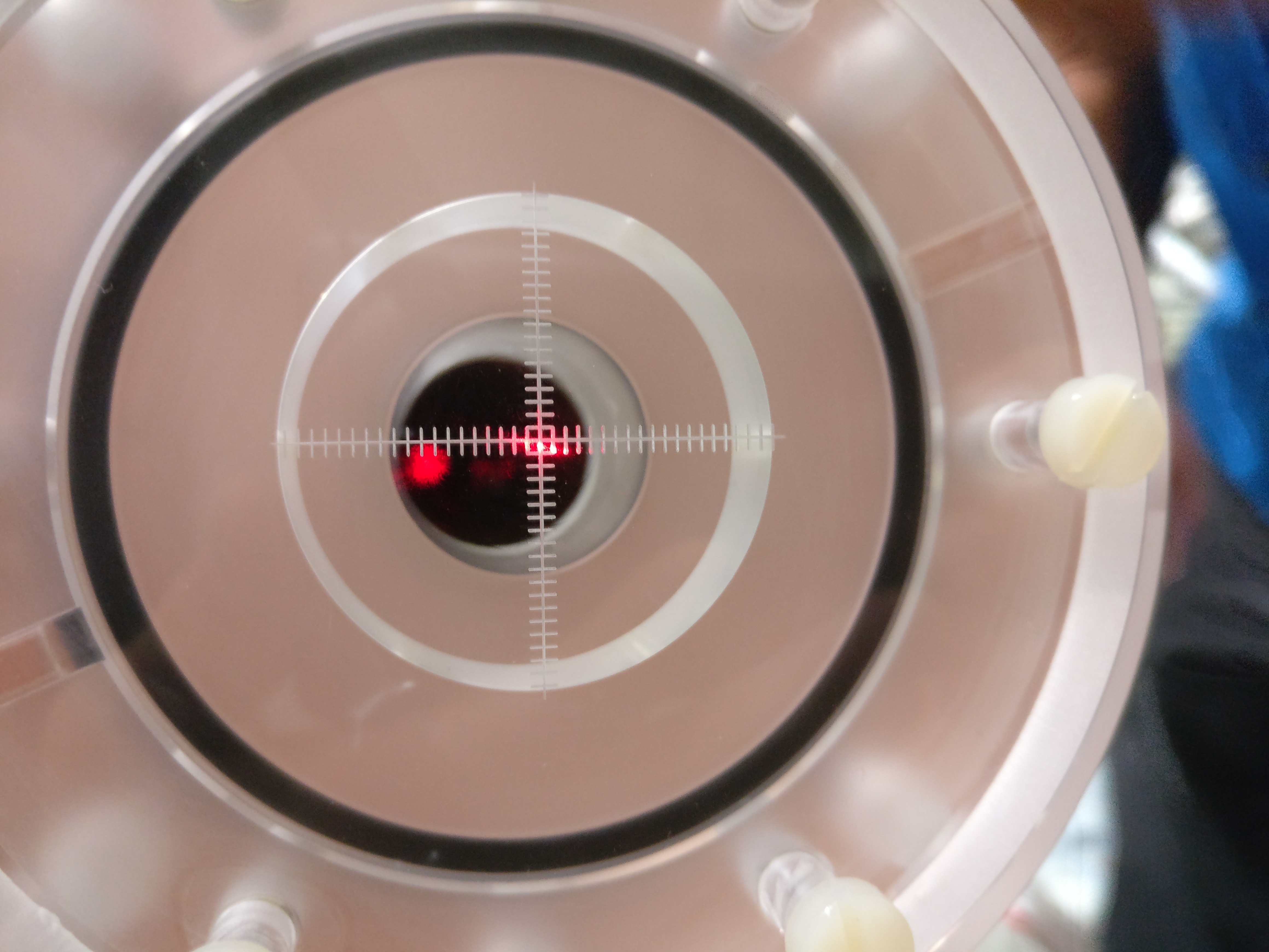
The Septemboard detector was prepared for data taking at the CAST experiment in July 2017 for preliminary alignment and fit tests. The detector beamline was prepared behind the LLNL telescope and aligned with a laser from the opposite side of the magnet using an acrylic glass target on (see fig. 1(a)). Vacuum leak tests were performed and the detector installed on (see fig. 1(b)). In addition, geometer measurements were done for final alignment and as a reference measurement the day after. An Amptek COOL-X X-ray generator 1 ('X-ray finger') was installed on the opposite side of the magnet. A calibration measurement with the X-ray finger ran from over night. The aim of an X-ray finger run is to roughly verify the focal spot of the X-ray telescope. After this initial test the detector was dismounted to make space for the KWISP experiment.
Two months later the detector was remounted between to with another geometer measurement on the last day. During an attempt to clean the detector water cooling system on , the window of the detector was destroyed (see section 10.4). This required a detector dismount and transport to Bonn for repairs as the detector was electronically dead after the incident.
Near the end of October the remount of the detector started and was finished by in time for another geometer measurement and alignment. The next day the veto paddle scintillator was calibrated using a 3-way coincidence in the RD51 laboratory (see sec. 8.3), followed by the installation of the lead shielding and scintillator installation another day later. With everything ready, data taking of the first data taking period with the Septemboard detector started on . During the period until few minor issues were encountered, see sec. 10.5.1. As CERN is typically closed over Christmas and well into January, data taking was paused until (further time is necessary to prepare the magnet for data taking again).
The second part of the first data taking then continued on until , with a few more small problems encountered, see 10.5.2. After data taking concluded, dismounting of the detector began the next day by removing the veto scintillator and the lead shielding. On another X-ray finger run was performed to get a sense of the placement of the detector during its actual mount as it was during the first data taking period. Afterwards, the detector was fully removed by to bring it back to Bonn to fix a few problems.
Data taking was initially intended to continue by summer of 2018. The fully repaired detector was installed between and with a few minor delays due to a change in mounting of the lead shielding support to accommodate a parallel data taking with KWISP. For alignment another geometer measurement was performed on . Unfortunately, external delays pushed the begin of the data taking campaign back into late October. On the data taking finally begins after a power supply issue was fixed the day before. The issues encountered during this data taking period, which lasted until are mentioned in sec. 10.5.3.
With the end of 2018 the data taking campaign of the Septemboard was at an end. The detector was moved over from CAST to the CAST Detector Lab (CDL) on for a measurement campaign behind an X-ray tube for calibration purposes. Data was taken until with a variety of targets and filters (covered in sec. 12.2 later). Afterwards the detector was dismounted and taken back to Bonn.
For the results of the different alignments, further see section 10.2.
10.1.1. Detailed technical timeline [/] extended
- Initial installation 2017
-
- ref:
https://espace.cern.ch/cast-share/elog/Lists/Posts/Post.aspx?ID=3420
and
~/org/Documents/InGrid_calibration_installation_2017_elog.pdf - June/July detector brought to CERN
- before alignment of LLNL telescope by Jaime
- laser alignment (see
 )
) - vacuum leak tests & installation of detector
(see:
)
- after installation of lead shielding
- Geometer measurement of InGrid alignment for X-ray finger run
- - : first X-ray finger run (not useful to determine position of detector, due to dismount after)
- after: dismounted to make space for KWISP
- ref:
https://espace.cern.ch/cast-share/elog/Lists/Posts/Post.aspx?ID=3420
and
- Installation for data taking start
-
- Remount in September 2017 -
- installation from to
- Alignment with geometers for data taking, magnet warm and under vacuum.
- Window explosion cleaning accident
-
- weekend: (ref: ./../org/Talks/CCM_2017_Sep/CCM_2017_Sep.html)
- calibration (but all wrong)
- water cooling stopped working
- next week: try fix water cooling
- quick couplings: rubber disintegrating causing cooling flow to go to zero
- attempt to clean via compressed air
- final cleaning : wrong tube, compressed detector…
- detector window exploded…
- show image of window and inside detector
- detector investigation in CAST CDL
see
 images & timestamps of images
 - study of contamination & end of Sep CCM
- detector back to Bonn, fixed
- weekend: (ref: ./../org/Talks/CCM_2017_Sep/CCM_2017_Sep.html)
- Reinstallation for data taking start (Run 2)
-
- detector installation before first data taking
- reinstall in October for start of data taking in 30th Oct 2017
- remount start
- Alignment with Geometers (after removal & remounting due to window accident) for data taking. Magnet cold and under vacuum.
- calibration of scintillator veto paddle in RD51 lab
- remount installation finished incl. lead shielding (mail "InGrid status update" to Satan Forum on )
- <data taking period from to in
2017>
- between runs 85 & 86: fix of
src/waitconditions.cppTOS bug, which caused scinti triggers to be written in all files up to next FADC trigger - run 101 was the first with FADC noise
significant enough to make me change settings:
- Diff: 50 ns -> 20 ns (one to left)
- Coarse gain: 6x -> 10x (one to right)
- run 109: crazy amounts of noise on FADC
- run 111: stopped early. tried to debug noise and blew a fuse in gas interlock box by connecting NIM crate to wrong power cable
- run 112: change FADC settings again due to noise:
- integration: 50 ns -> 100 ns This was done at around
- integration: 100 ns -> 50 ns again at around .
- run 121: Jochen set the FADC main amplifier integration time from 50 -> 100 ns again, around
- between runs 85 & 86: fix of
- <data taking period from to
beginning 2018>
- start of 2018 period: temperature sensor broken!
- to issues with moving THL values & weird detector behavior. Changed THL values temporarily as an attempted fix, but in the end didn't help, problem got worse. (ref: gmail "Update 17/02" and ./../org/Mails/cast_power_supply_problem_thlshift/power_supply_problem.html) issue with power supply causing severe drop in gain / increase in THL (unclear, #hits in 55Fe dropped massively ; background eventually only saw random active pixels). Fixed by replugging all power cables and improving the grounding situation. iirc: this was later identified to be an issue with the grounding between the water cooling system and the detector.
- by everything was fixed and detector was running correctly again.
-
2 runs:
were missed because of this.
- removal of veto scintillator and lead shielding
- X-ray finger run 2 on . This run is actually useful to determine the position of the detector.
- Geometer measurement after warming up magnet and not under vacuum. Serves as reference for difference between vacuum & cold on !
- detector fully removed and taken back to Bonn
- Reinstallation for data taking in Oct 2018 (Run 3)
-
- installation started . Mounting due to lead shielding support was more complicated than intended (see mails "ingrid installation" including Damien Bedat)
- shielding fixed by and detector installed the next couple of days
- Alignment with Geometers for data taking. Magnet warm and not under vacuum.
- data taking was supposed to start end of September, but delayed.
- detector had issue w/ power supply, finally fixed on . Issue was a bad soldering joint on the Phoenix connector on the intermediate board. Note: See chain of mails titled "Unser Detektor…" starting on for more information. Detector behavior was weird from beginning Oct. Weird behavior seen on the voltages of the detector. Initial worry: power supply dead or supercaps on it. Replaced power supply (Phips brought it a few days after), but no change.
- data taking starts
- run 297, 298 showed lots of noise again, disabled FADC on (went to CERN next day)
- data taking ends
-
runs that were missed:
The last one was not a full run.
-
[ ]CHECK THE ELOG FOR WHAT THE LAST RUN WAS ABOUT
- CAST Detector Lab measurements
-
- detector mounted in CAST Detector Lab
- data taking from to .
- detector dismounted and taken back to Bonn
- Outer chip 55Fe calibrations
-
- ref: ./../org/outerRingNotes.html
- calibration measurements of outer chips with a 55Fe source using a custom anode & window
- between and calibrations of each outer chip using Run 2 and Run 3 detector calibrations
- start of a new detector calibration
- another set of measurements between to with a new set of calibrations
10.2. Alignment
Detector alignment with the X-ray telescope, the magnet and by extension the solar core during solar tracking is obviously crucial for a helioscope for a good physics result. The alignment procedure used for the Septemboard detector is a three-fold approach:
- alignment of the piping up to the detector using an acrylic glass target with a millimeter spaced cross, as seen in fig. 1(a). This target is mounted to the vacuum pipes in the same way the detector is mounted. A laser is installed on the opposite side of the magnet. With the magnet bores fully open the laser is aligned such that it propagates the full bore and is reflected by the X-ray telescope into the focal spot. This alignment guarantees the focal spot location to be near the center of the detector. Uncertainty is introduced due to the need to remove the acrylic glass target and install the detector, as the mounting screws allow for small movements. In addition the vacuum pipes are also not perfectly fixed.
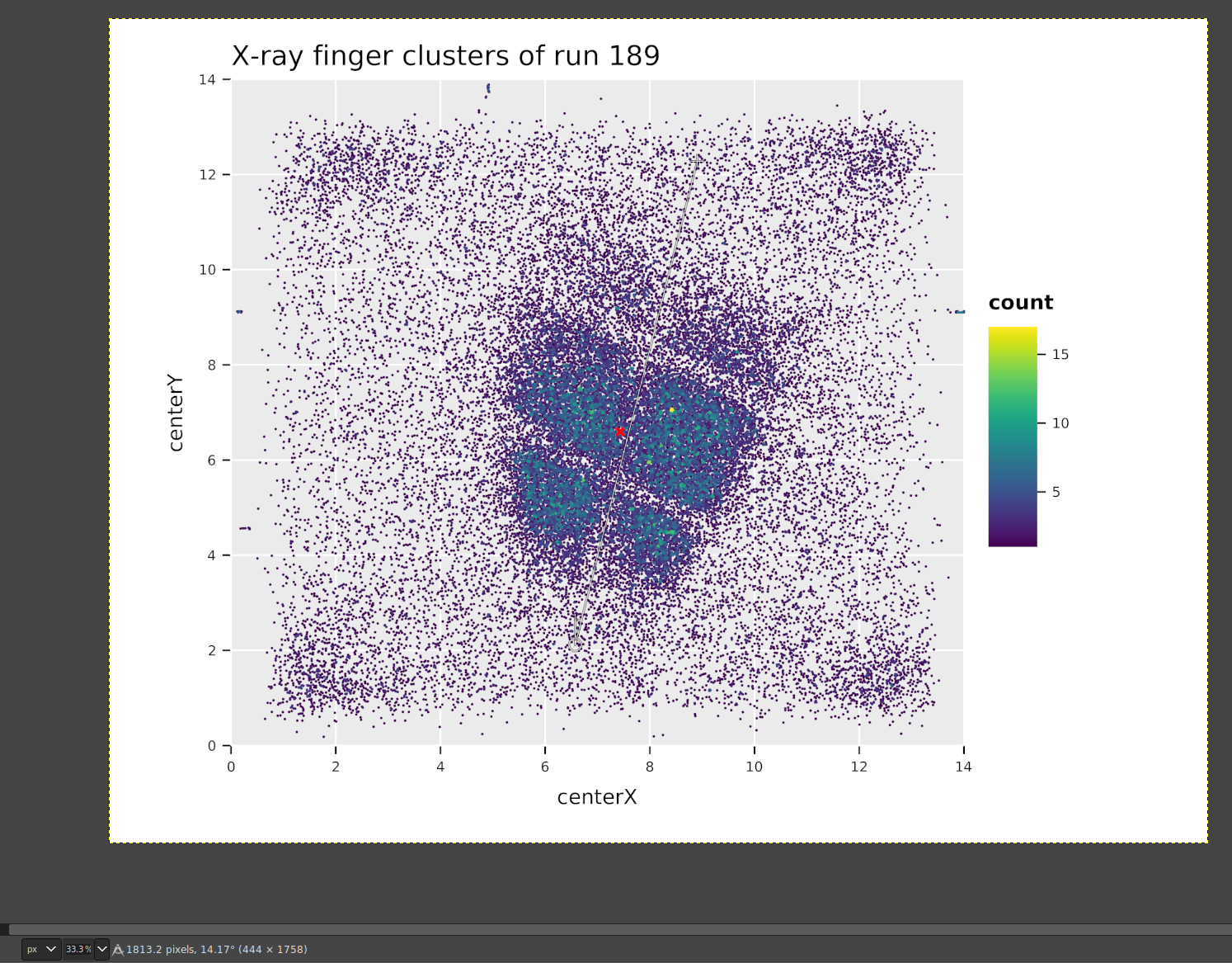
- alignment of the fully installed detector using an X-ray finger. The 'X-ray finger' is a small electric X-ray generator (in particular an Amptek COOL-X), which is installed in the magnet bore at the opposite end of the magnet. The generated X-rays must traverse the magnet and telescope, thereby being focused by the telescope into the focal spot. As the X-ray finger does not emit parallel light, the resulting distribution of the X-rays on the detector is not a perfect focal spot, even if the telescope was perfect and the detector placed right in the focus. The close distance also implies the focal length is slightly different than for an infinite source. The mean position of the taken data can anyhow be used to determine the likely focal spot position. See below, fig. 2(a), for an example and the resulting position from one of the X-ray finger runs.
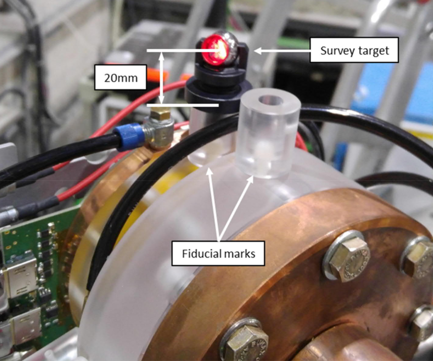
- alignment by the geometer group at CERN. A theodolite is installed in the CAST hall and the location of many targets on the magnet, telescope, vacuum pipes and the detector itself are measured up to \(\SI{0.5}{mm}\) precision at \(1σ\) level. See fig. 2(b) for a picture of such a target. The initial geometer measurement from mainly serves as a baseline reference. As the first two alignment procedures provide a good alignment, a measurement of the existing position by the geometers can then later be used to re-align the detector after it was removed relative to the previous baseline position relative to the telescope. This assures the detector can be remounted and placed in the right location without the need for an additional laser alignment.
The X-ray finger run taken in April 2018 can be used as a reference for the alignment as used during the first data taking. The center positions of each cluster can be shown as a heatmap, where the number of hits each pixel received is colored. Computing the mean position of all those clusters yields the most likely center position of the focal spot. See fig. 2(a) for an example of this. The position of the center based on the mean of all cluster centers is about \(\SI{0.4}{mm}\) away from the center in both axes.

With this setup after each remounting a geometer measurement was performed to align the detector back to the initial laser alignment. As the second mounting of the detector in September 2017 was not used for any data taking, the associated geometer measurement is irrelevant.
Tab. 11 summarizes the values of the geometer alignment results for each of the measurements using the CenterR and CenterF positions defined based on the initial geometer measurement in July 2017. In each case the shifts in X, Y and Z direction is usually significantly less than \(\SI{1}{mm}\).
| Measurement | Target | ΔX [mm] | ΔY [mm] | ΔZ [mm] | Useful |
|---|---|---|---|---|---|
| 11.07.2017 | yes | ||||
| 14.09.2017 | CenterR | -0.1 | 0.3 | -0.8 | no |
| CenterF | -0.1 | 0.3 | -0.9 | ||
| 26.10.2017 | CenterR | 0.2 | 0.6 | 0.2 | yes |
| CenterF | 0.1 | 0.6 | -0.1 | ||
| 24.04.2018 | CenterR | 0.5 | 0.5 | 0.0 | yes |
| CenterF | 0.4 | 0.5 | -0.3 | ||
| 23.07.2018 | CenterR | 1.1 | 0.5 | 0.6 | yes |
| CenterF | 1.0 | 0.5 | 0.3 |
For a detailed overview of the geometer measurements see the public EDMS links under (B. C. Antje Behrens 2017; B. C. Antje Behrens Alexandre Beynel 2017a, 2017b; Antje Behrens 2018b, 2018a) containing the PDF reports for each measurement.
10.2.1. Some extra info about the geometer alignment extended
The following is the snippet from the PDF report about the definition of the CenterR and CenterF positions.
Goal of the operation has been to align the InGRID detector with respect to the LLNL telescope as on 11.07.2017 after the alignment of the setup with respect to the LASER installed. Coordinates of the measurement on 11.07.2017 are given below.
In order to compare InGRID position on 11.07 and 14.09, two points close to the detector axis CenterR and CenterF have been defined on 11.07. Afterwards their coordinates for the measurement on 14.09 have been calculated.
10.2.2. Generate X-ray heatmap [/] extended
[X]FIND XRAY FINGER RUN 2, RUN 189! ./../CastData/data/XrayFingerRuns/[X]RECREATE BELOW FOR THE OTHER XRAY FINGER RUN! -> Both are created and listed below.[ ]RECREATE PLOTS AS TIKZ + VEGA -> We create them on the Cairo backend using DejaVu Serif, same as in the document of the thesis now. This is because the TikZ produced vector graphic ends up much larger than the Cairo one. Vega is on hold for now.[X]VERIFY THAT WE (LIKELY) HAVE TO ROTATE THE DATA BY 90 DEGREES AS ONE OF THE VERTICAL LINES IS THE TELESCOPE AXIS WHICH SHOULD BE HORIZONTAL TO THE GROUND -> Yes, we do.
First let's reconstruct the X-ray finger run:
    import shell, strutils

proc main  (path: string, run: int  ) =
  #   parse data
  let outfile = "/t/xray_finger_  $#  .h5" % $run
  let recoOut = "/t/reco_xray_finger_  $#  .h5" % $run

  shell:
    raw_data_manipulation -p ($path) "--runType xray --out " ($outfile)
  shell:
    reconstruction -i ($outfile) "--out " ($recoOut)

when isMainModule:
  import cligen
  dispatch main
And now we simply create a heatmap of the cluster centers:
    import nimhdf5, ggplotnim, options
import ingrid / tos_helpers
import std / [strutils, tables]

proc main  (run: int, switchAxes: bool = false, useTeX = false  ) =
  let file = "/t/reco_xray_finger_  $#  .h5" % $run

  #  proc readClusters(h5f: H5File): (seq[float], seq[float]) =
  var h5f = H5open  (file, "r"  )

  #   compute counts based on number of each pixel hit
  proc toIdx  (x: float  ): int = (x / 14.0 * 256.0  ).round.int.clamp  (  0, 255  )
  var ctab = initCountTable[  (  int, int  )  ]()

  var df = readRunDsets(h5f, run = run,
                        chipDsets = some(  (
                        chip: 3, dsets: @[  "centerX", "centerY"  ]  )  )  )
    .mutate(f{  "xidx" ~ toIdx(idx(  "centerX"  )  )  },
            f{  "yidx" ~ toIdx(idx(  "centerY"  )  )  }  )
  let xidx = df[  "xidx", int  ]
  let yidx = df[  "yidx", int  ]
  forEach x in xidx, y in yidx:
    inc cTab, (x, y)
  df = df.mutate(f{  int: "count" ~ cTab[  (`xidx`, `yidx`)  ]  }  )
  let centerX = df[  "centerX", float  ].mean
  let centerY = df[  "centerY", float  ].mean
  discard h5f.close  ()

  echo "Center position of the cluster is at: (x, y) = (", centerX, ", ", centerY, ")"
  ## NOTE: Exchanging the axes for X and Y is equivalent to a 90° clockwise rotation for our data
  ## because the centerX values are inverted `  (256 - x), applyPitchConversion  `.
  ## The real rotation of the Septemboard detector at CAST seen from the telescope onto the
  ## detector is precisely 90° clockwise.
  let x = if switchAxes: "centerY" else: "centerX"
  let y = if switchAxes: "centerX" else: "centerY"
  let cX = if switchAxes: centerY else: centerX
  let cY = if switchAxes: centerX else: centerY
  ggplot(df, aes(x, y, color = "count"  )  ) +
    geom_point(size = 0.75  ) +
    geom_point(data = newDataFrame(), aes = aes(x = cX, y = cY),
               color = "red", marker = mkRotCross) +
    scale_color_continuous() +
    ggtitle(  "X-ray finger clusters of run   $#  " % $run) +
    xlab(r"x [mm]"  ) + ylab(r"y [mm]"  ) +
    xlim(  0.0, 14.0  ) + ylim(  0.0, 14.0  ) +
    margin(right = 3.5  ) +
    #  theme_scale(1.0, family = "serif") +
    coord_fixed(  1.0  ) +
    themeLatex(fWidth = 0.5, width = 600, baseTheme = sideBySide) +
    legendPosition(  0.83, 0.0  ) +
    ggsave(  "/home/basti/phd/Figs/CAST_Alignment/xray_finger_centers_run_  $#  .pdf" % $run,
           useTeX = useTeX, standalone = useTeX, dataAsBitmap = true  )
           #  useTeX = true, standalone = true)

when isMainModule:
  import cligen
  dispatch main
First perform the data reconstruction:
  ./code/xray_finger_data_parsing -p ~/CastData/data/XrayFingerRuns/Run_21_170713-11-03 --run 21
./code/xray_finger_data_parsing -p ~/CastData/data/XrayFingerRuns/Run_189_180420-09-53 --run 189
And now create the plots:
  ./code/xray_finger_center_plot -r 21 --switchAxes
./code/xray_finger_center_plot -r 189 --switchAxes
For run 21: Center position of the cluster is at: (x, y) = (7.210714052855218,5.669514297250704) For run 189: Center position of the cluster is at: (x, y) = (7.428075467697270,6.594113570730057)
First the plot for the (unused) X-ray finger run taken at the first
installation before any data taking (detector removed afterwards):

And second the plot of the 2018 X-ray finger run taken before the detector was removed in Apr 2018. This is the baseline for our idea where the focal spot is going to be. Figs/CAST_Alignment/xray_finger_centers_run_189.pdf
NOTE: For a longer explanation about the reasoning behind the
comment for --switchAxes in the code, see
sec. 13.14.7.
10.2.3. Generate spectrum of X-ray finger run extended
Let's also look at the spectrum of the X-ray finger run (at least 189).
Given the reconstructed H5 file of the run 189
  plotBackgroundRate \
    \t\reco_xray_finger_189.h5 \
    --names "X-ray finger" \
    --title "X-ray finger run 189 spectrum" \
    --centerChip 3 \
    --region crGold \
    --energyDset energyFromCharge \
    --outfile xray_finger_spectrum_189.pdf \
    --outpath ~/phd/Figs/XrayFinger/ \
    --useTeX \
    --quiet
Which yields the following figure:

10.2.4. Systematic uncertainty from graphite spacer rotation [/] extended
[X]Determine the rotation angle of the graphite spacer from the X-ray finger data -> do now. X-ray finger run:
->
 -> It comes out to 14.17°!
But for run 21 (between which detector was dismounted of course):
-> It comes out to 14.17°!
But for run 21 (between which detector was dismounted of course):
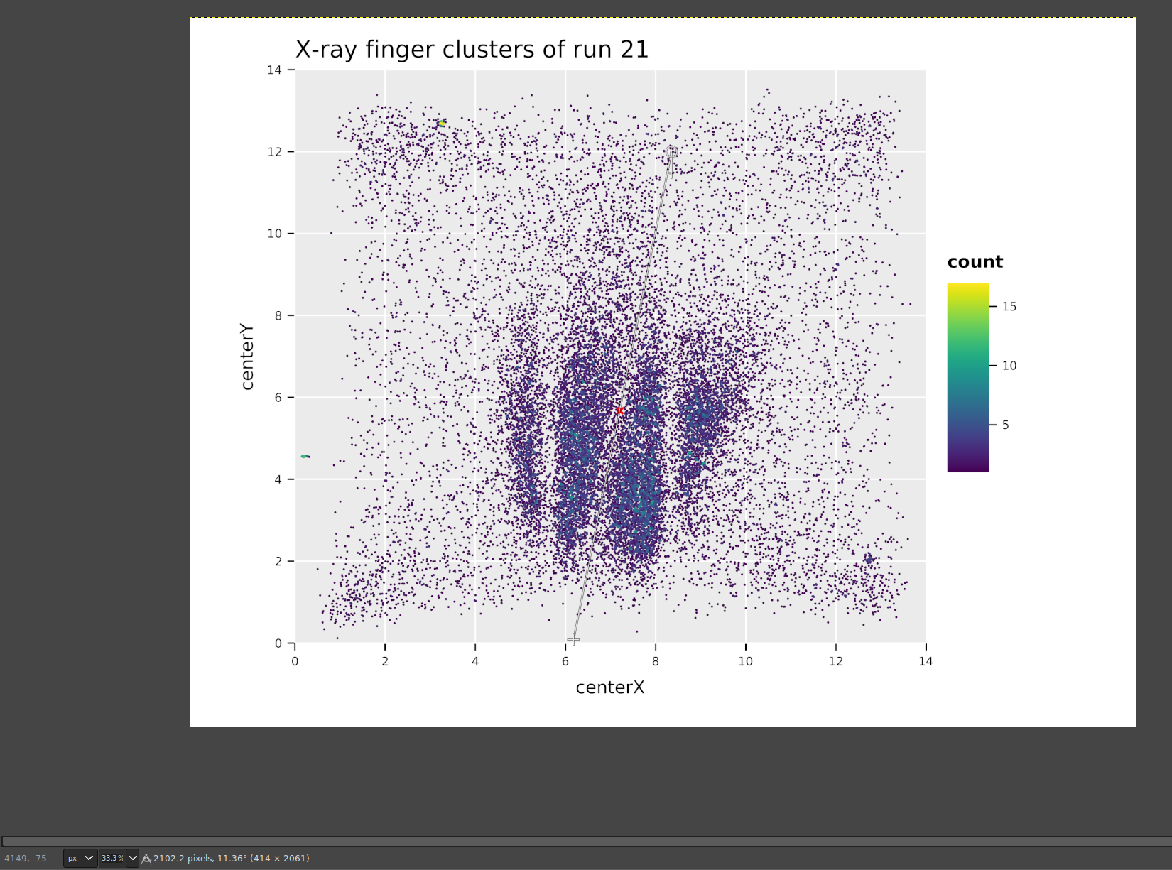 -> Only 11.36°!
That's a huge uncertainty given the detector was only dismounted!
3°.
-> Only 11.36°!
That's a huge uncertainty given the detector was only dismounted!
3°.[ ]rotation of telescope![ ]Effect on systematic uncertainty!
10.3. Detector setup at CAST
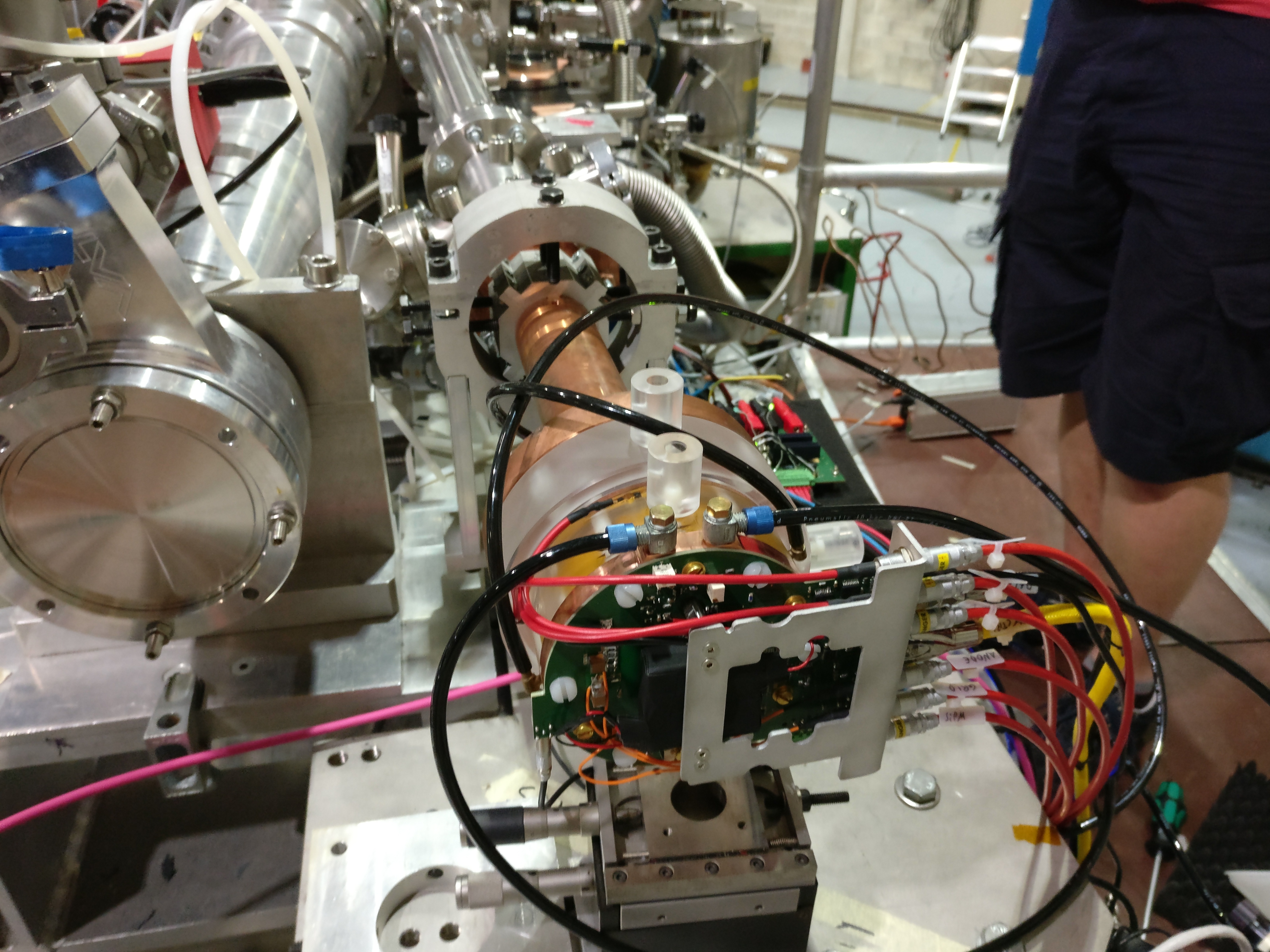
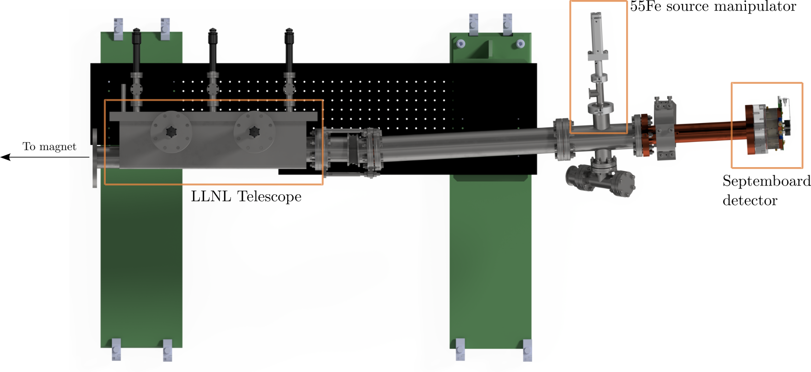
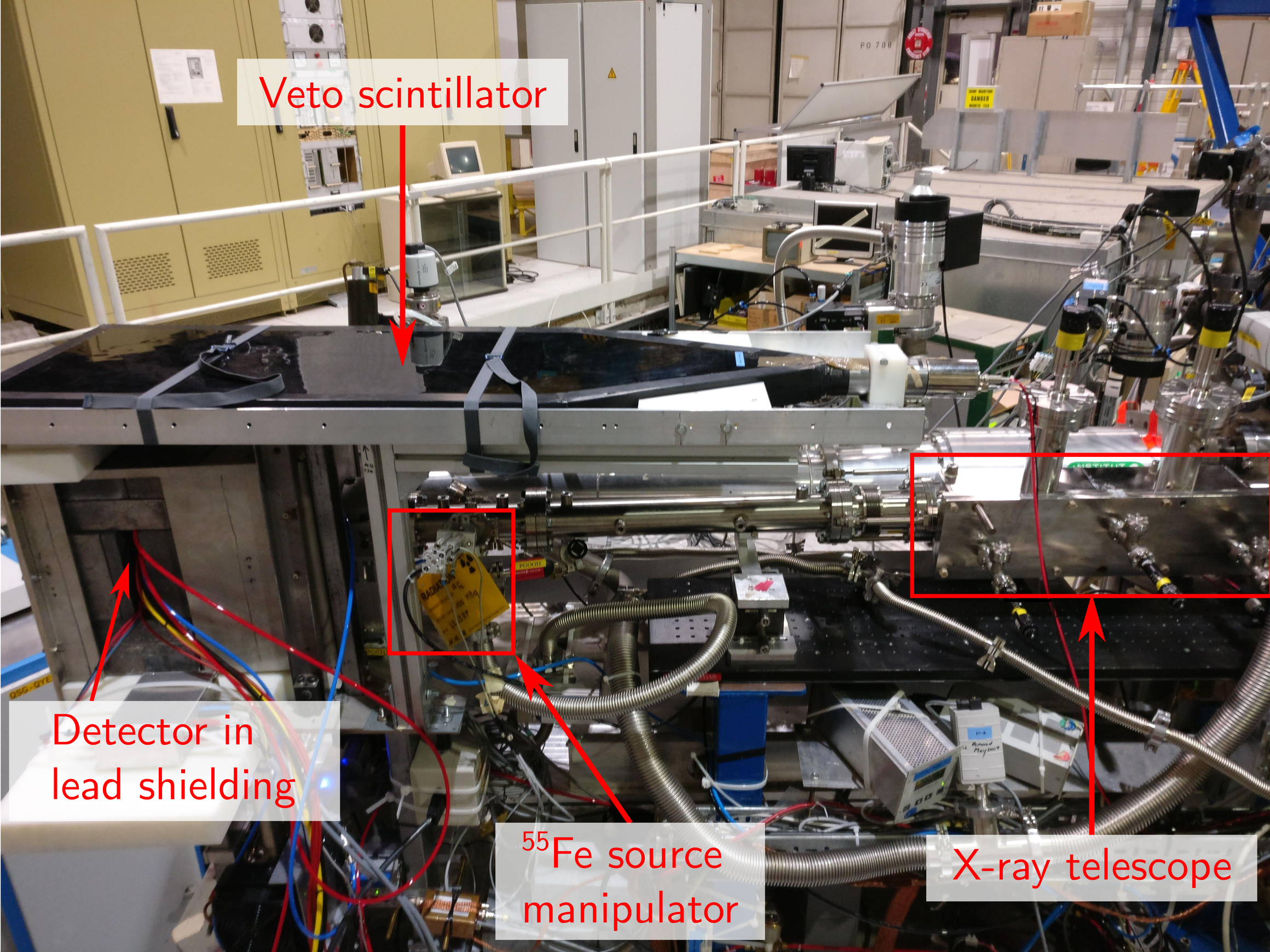
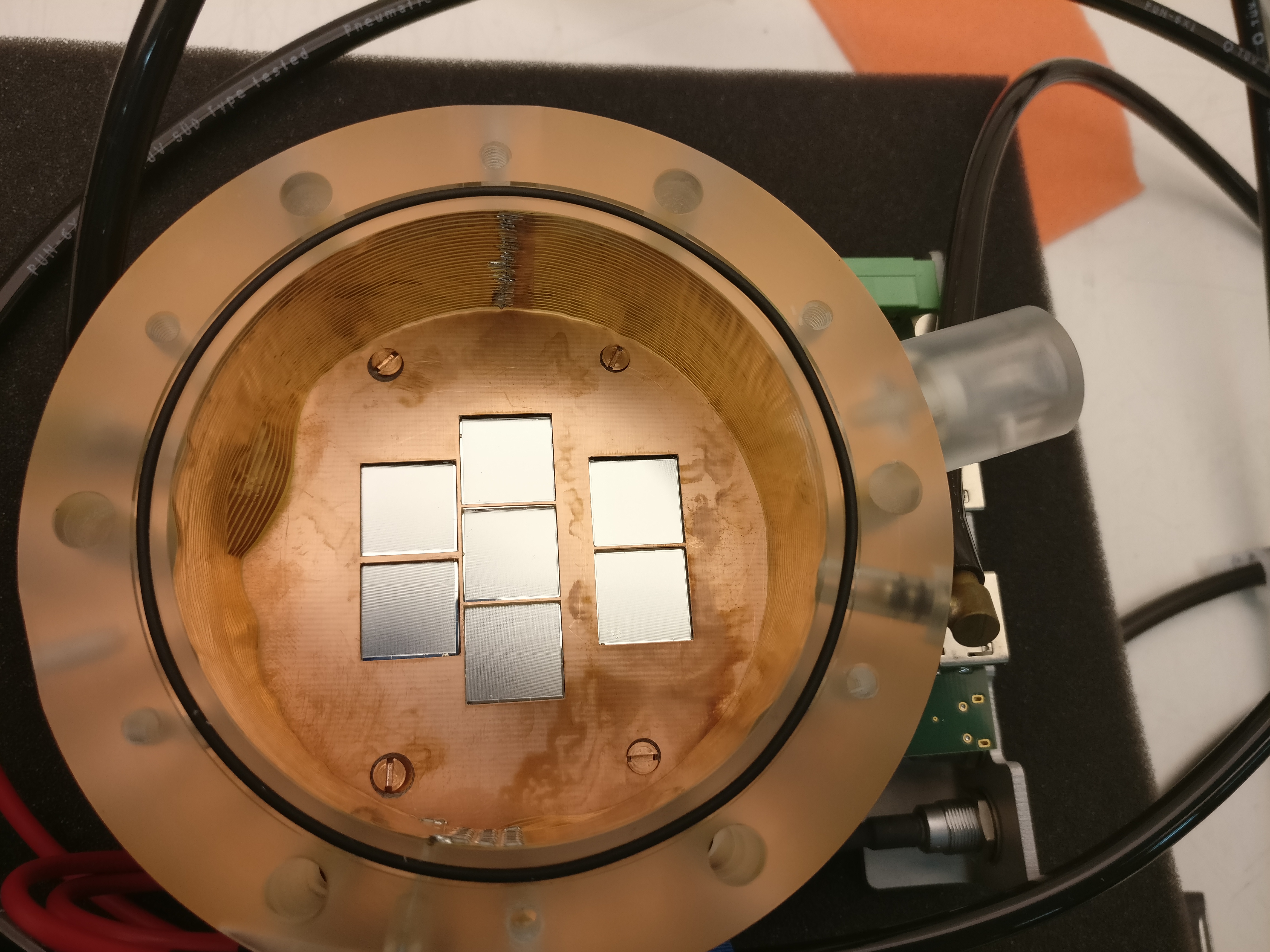
The setup of the full beamline from the magnet end cap to the detector is shown in a render in fig. 4. The piping shows a clear kink introduced using a flexible bellow. This setup is used to move the detector mount further away from the other beamline to provide more space for two setups side-by-side. At the same time it is an artifact of the LLNL telescope only being a \(\SI{30}{°}\) portion of a full telescope resulting in the focal plane not being centered in front of the telescope. Not shown in the image is the lead shielding installed around the detector as well as the veto scintillator, which covers the majority of the beamline area. The lead shielding is a \(\SIrange{5}{15}{cm}\) thick 'castle' of lead around the detector (\(\SI{10}{cm}\) on top and behind, \(\SI{15}{cm}\) in front and \(\SI{5}{cm}\) and \(\SI{10}{cm}\) on each side). An annotated image of the real setup is seen in fig. 5, which shows lead shielding, veto scintillator, \cefe source manipulator and the LLNL X-ray telescope. The setup is behind the VT3 gate valve of the CAST magnet.
10.3.1. \cefe source and manipulator
As seen in the previous section the setup includes a \cefe source. Its purpose is both monitoring of the detector behavior and it serves as a way to calibrate the energy of events (as mentioned in theory section 6.3.8). More details on the usage and importance for data analysis will be given in chapter 11. It is installed on a pneumatic manipulator. Using a compressed air line with about \(\SI{6}{bar}\) pressure the manipulator can be moved up and down. Under vacuum conditions of the setup the manipulator is inserted unless the compressed air is used to push it out.
A Raspberry Pi 2 is installed close to the manipulator and connects to the two Festo 3 control sensors at the top and bottom end of the manipulator using the general purpose input/output (GPIO) pins. Two pins are used to read the sensor status from each. Five more pins connect to a \(\SI{24}{V}\) relay, which is used to control the controllers for the compressed air line. The relay is controlled by pulse width modulation (PWM). The software controlling the GPIO pins of the Raspberry Pi is written in Python. A client program is running on a computer in the CAST control room and communicates with the Raspberry Pi using a network connection on which a server process is running. It can receive connections through a socket, allowing for remote and programmatic control of the manipulator via a set of simple string based messages. Further, it provides a REPL (read-evaluate-print loop) to control it interactively. For more details about the software see the extended version of this thesis.
10.3.1.1. Manipulator software and notes [0/1] extended
[ ]MOVE MANIPULATOR CODE TO TPA TOOLS AND LINK TO IT? -> Code can definitely go to TPA repository. The notes I think are enough if they are simply added as an Org file into the repository as well. They are too specific in some sense?
The source code of the python script running on the Raspberry Pi to control the manipulator is the following script:
    #  !/usr/bin/env python3.6

import sys
import pigpio
import readline
import logging
import argparse
import time
import socket
import threading
import json
import asyncio
import functools
import weakref

#   the program needs to do the following
#
#   - on RPi 7 pins used (5 controlled via software):
#       - relay:
#           - GOOD  - input, Pin 14
#           - OUT   - input, Pin 15
#           - RC IN - output (via PWM), via Pin 14
#           - VRC   - const voltage, using 5V via PIN 2, not done in software
#           - GND   - ground, pin 6, not done in software
#       - sensors 2 pins:
#           - input, read sensor output
#
#
#   program always listens to GOOD and OUT
#   using PWM we activate the manipulator. done by waiting for
#    - command line input?
#    - reading some file, s.t. this program runs as a daemon and we use
#      some external tool to write file via usb to Pi
#    - finally be able to execute from TOS. easiest via script to call
#   reading sensor inputs done in connection with usage of PWM
#
#   finally compile this program to jar to run it


#   in order to control the source via network, the basic usage is something like
#   the following:
#   s = socket.socket(socket.AF_INET, socket.SOCK_STREAM)
#   s.connect(('localhost', 42000))
#   s.send("insert".encode())
#   depening on whether the call is from the local machine or not.
#   "insert" and "remove" are supported at the moment
#   sends back a byte string containing the bool of the
#   insertion / removal

#  class client(asyncio.Protocol):


#   connect to pi at IP address
p = pigpio.pi(  '10.42.0.91'  )

#   define dict of pins
d = {  "GOOD"    : 14,
     "OUT"     : 15,
     "RC_IN"   : 18,
     "S_OPEN"  : 20,
     "S_CLOSE" : 21}


class server  (threading.Thread):
    #   this is a simple server class, which receives the necessary
    #   parameters to control the raspberry pi and a socket, from
    #   which it listens to commands
    #   inherits from threading.Thread to run in a separate thread

    def __init__  (  self, socket, p, d, pwm):
        #   init the object
        self.socket = socket
        self.p      = p
        self.d      = d
        self.pwm    = pwm
        self._stop  = False
        #   now call the Thread init
        threading.Thread.__init__(  self  )
        #   and set it as a daemon, so that it cannot
        #   stop the main program from quitting
        self.setDaemon(  True  )

    async def process_client  (  self, reader, writer):
        client = writer.get_extra_info(  'peername'  )
        print  (  "New client connected: {}".format  (client)  )
        while self._stop == False:
            #  data = socket.recv(1024).decode()
            data = (  await reader.readline()  ).decode()
            if data:
                success = self.parse_message(data, client)
                message = self.create_message(client[0], success)
                writer.write(message)
                await writer.drain()
            else:
                writer.close()
                break

    #   hacky get loop...
    def get_loop_and_server  (  self  ):
        return (  self.loop, self.socketserver)

    def run  (  self  ):
        #   using run we start the thread

        #   need a new event loop, in which asyncio works
        self.loop = asyncio.new_event_loop()
        asyncio.set_event_loop(  self.loop)
        #   start server on specific port open on all interfaces
        self.server_future = asyncio.start_server(  self.process_client, host = "0.0.0.0", port = 42000)
        #   the returned future is handed to the event loop
        self.socketserver = self.loop.run_until_complete(
            asyncio.ensure_future(
                self.server_future,
                loop = self.loop)  )

        print  (  self.socketserver.sockets)
        #   run
        self.loop.run_forever()

    def stop_server  (  self  ):
        #   in case stop_server is called, the stop flag is
        #   set, such that the while loop, which waits for
        #   data from the socket stops
        self._stop = True

        while self.loop.is_running() == True:
            print  (  "current sockets still connected {}".format  (  self.socketserver.sockets)  )
            print  (  "loop is still running: {}".format  (  self.loop.is_running()  )  )

            #  self.socketserver.wait_closed()
            self.loop.stop()
            self.server_future.close()
            self.socketserver.close()
            #   next line raises an exception, loop still running....
            #   TODO: fix problem that we cannot stop the running event loop :(
            self.loop.close(  self.loop.run_until_complete(  self.socketserver.wait_closed()  )  )
            time.sleep(0.2)

        self.loop.close()


    def parse_message  (  self, data, address):
        #   this function parses the data. If there is a function
        #   call in the data, we call the appropriate function
        ip, port = address
        result = False
        if 'insert' in data:
            result = insert_source(  self.p, self.d, self.pwm)
            #  logging.info("source inserted via network socket {}:{}".format(ip, port))
        elif 'remove' in data:
            result = remove_source(  self.p, self.d, self.pwm)
            #  logging.info("source removed via network socket {}:{}".format(ip, port))
        elif 'out?' in data:
            result = read_out(  self.p, self.d)
            #  logging.info("out? status requestet via network socket {}:{}".format(ip, port))
        elif 'good?' in data:
            #   read GOOD and print
            result = read_good(  self.p, self.d)
            #  logging.info("good? status requestet via network socket {}:{}".format(ip, port))
        elif 's_open?' in data:
            #   read sensor 1 and print
            result = read_sensor_open(  self.p, self.d)
            #  logging.info("s_open? status requestet via network socket {}:{}".format(ip, port))
        elif 's_close?' in data:
            #   read sensor 1 and print
            result = read_sensor_close(  self.p, self.d)
            #  logging.info("s_close? status requestet via network socket {}:{}".format(ip, port))
        else:
            result = "Unknown command"

        return result

    def create_message  (  self, client, data):
        #   this function creates a JSON message containing the returned value
        #   of the RPi call and a clientname
        #   using dictionary, we create a json dump and return the encoded
        #   string
        message = {  "username" : client, "message" : data}
        #   add trailing \r\l to indicate end of data stream
        json_data = json.dumps(message) + '  \n  '
        return json_data.encode()


#   set relay_sleep time (time to wait for activation of relay): 50ms
relay_sleep = 50e-3
#   set manipulator_sleep time: 1s
manip_sleep = 1

def print_help  ():

    help_string = """
    The following commands are available:  \n
        insert : insert source into bore
        remove : remove source from bore
        out?   : print current value of relay OUT
        good?  : print current value of relay GOOD
        d?     : parameters used for relay (pin layout etc.)
        pwm?   : parameters used for PWM (frequency, duty cycle, ...)
        help   : prints this help
    """

    print  (help_string)
    return


def read_good  (p, d):
    #   simple function which returns the value of the
    #   GPIO pin for the GOOD output of the relay
    good = bool  (p.read(d[  "GOOD"  ]  )  )
    return good

def read_out  (p, d):
    #   simple function which returns the value of the
    #   GPIO pin for the OUT output of the relay
    out = bool  (p.read(d[  "OUT"  ]  )  )
    return out

def read_sensor_open  (p, d):
    #   simple function which returns bool corresponding to
    #   GPIO pin of sensor for OPEN
    val = bool  (p.read(d[  "S_OPEN"  ]  )  )
    return val

def read_sensor_close  (p, d):
    #   simple function which returns bool corresponding to
    #   GPIO pin of sensor for CLOSED
    val = bool  (p.read(d[  "S_CLOSE"  ]  )  )
    return val

def configure_pins  (p, d):
    #   function to export all pins and set to correct modes
    #   relay control / reading
    p.set_mode(d[  "GOOD"  ], pigpio.INPUT)
    p.set_mode(d[  "OUT"  ], pigpio.INPUT)
    p.set_mode(d[  "RC_IN"  ], pigpio.OUTPUT)
    #   sensor reading
    p.set_mode(d[  "S_OPEN"  ], pigpio.INPUT)
    p.set_mode(d[  "S_CLOSE"  ], pigpio.INPUT)
    return

def pwm_control  (p, d, freq, duty_cycle):
    #   function to control the pwm of the RC IN pin
    p.hardware_PWM(d[  "RC_IN"  ], freq, duty_cycle)
    return

def insert_source  (p, d, pwm):
    #   inserts the source into the bore by activating the relay
    #   wrapper for source_control
    success = source_control(p, d, pwm, "on"  )
    return success

def remove_source  (p, d, pwm):
    #   removes source from bore by disabling the relay
    #   wrapping source control
    success = source_control(p, d, pwm, "off"  )
    return success

def source_control  (p, d, pwm, direction):
    #   this function provides a generalized interface to control the source
    #   inputs:
    #       p: the Pi object
    #       d: the dict. containing the parameters
    #       pwm: the dict. containing pwm parameters
    #       direction: a string describing the direction to move the source
    #           "on"  : insert source
    #           "off" : remove source


    pwm_control(p, d, pwm[  "f"  ], pwm[direction]  )
    #   relay was triggered: means relay should now read
    #   insert:
    #   GOOD == True &
    #   OUT  == True
    #   remove:
    #   GOOD == True &
    #   OUT  == False
    time.sleep(relay_sleep)
    good = read_good(p, d)
    out  = read_out(p, d)
    success = False

    #   set expected values based on insertion / removal
    if direction == "on":
        good_exp = True
        out_exp  = True
    elif direction == "off":
        good_exp = True
        out_exp  = False
    else:
        raise NotImplementedError  (  "only 'on' and 'off' implemented to control source."  )

    s1 = None
    s2 = None
    if good == good_exp and out == out_exp:
        #   if good is True and out False, everything fine
        #  logging.debug("pwm set to {}, relay reports: (good : {}), (out : {})".format(direction, good ,out))
        #   after setting of relay, wait again and check sensors
        print  (  'pwm switched, waiting for manipulator to be moved'  )
        time.sleep(manip_sleep)
        #   check sensors
        s1 = read_sensor_open(p, d)
        s2 = read_sensor_close(p, d)

        #  logging.debug('sensors report: s1 = {}, s2 = {}'.format(s1, s2))
        #   TODO: implement logic, which deals with sensors of manipulators

        if direction is "on":
            #   after insertion the sensors should read:
            #   s1 (sensor open) == True
            #   s2 (sensor close) == False
            if s1 == True and s2 == False:
                success = True
            else:
                success = False
        else:
            if s1 == False and s2 == True:
                #   after removal the sensors should read:
                #   s1 (sensor open) == False
                #   s2 (sensor close) == True
                success = True
            else:
                success = False

        if success == False:
            #  logging.warning("""WARNING: direction was {}, but sensors read (open): {} (close): {}.
            #  Relay switched correctly.""".format(direction, s1, s2))
            pass

    elif good == good_exp and out != out_exp:
        #   something is wrong, seems like relay did not change, both still repot True
        #  logging.warning("pwm set to {}, relay good, but OUT still reports True: {}, {}".format(direction, good, out))
        pass
    elif good == False:
        #  logging.warning("relay reports bad signal: {}".format(good))
        pass
    else:
        #  logging.warning("should not happen. Contact developer.")
        pass

    if direction == "on":
        print  (  "Insertion returned {}".format  (success)  )
        if success == False:
            print  (  "WARNING: insertion may have failed, but sensors read (open): {} (close): {}".format  (direction, s1, s2)  )
            print  (  "However, relay was activated correctly."  )
    elif direction == "off":
        print  (  "Removal returned {}".format  (success)  )
        if success == False:
            print  (  "WARNING: removal may have failed, but sensors read (open): {} (close): {}".format  (direction, s1, s2)  )
            print  (  "However, relay was activated correctly."  )


    #   the following lines are here to make sure there is a new prompt
    #   even in case a network call was made before
    sys.stdout.write(  '> '  )
    sys.stdout.flush()

    return success

def control_loop  (p, d, pwm):
    #   this function defines the main control loop of the manipulator
    #   control
    print  (  'Starting command prompt'  )
    print  (  '  \t   insert : inserts source into bore'  )
    print  (  '  \t   remove : removes source out of bore'  )
    print  (  '  \t   quit   : stop the program'  )

    #   TODO: still need to implement the checks for
    #         - sensor positions
    #           output warning to console and log file in case sensors
    #           don't report what was commanded
    #         - output warning in case signal not good

    while True:
        #   the sys calls are used to make sure the line is empty before we
        #   write to it via input. Don't want two > > to appear (depening
        #   on network calls this might happen)
        sys.stdout.write(  '  \r  '  )
        sys.stdout.flush()
        line = input  (  '> '  )
        if 'insert' in line:
            insert_source(p, d, pwm)
            #  logging.info("source inserted")
        elif 'remove' in line:
            remove_source(p, d, pwm)
            #  logging.info("source removed")
        elif 'out?' in line:
            #   read OUT and print
            print  (read_out(p, d)  )
        elif 'good?' in line:
            #   read GOOD and print
            print  (read_good(p, d)  )
        elif 's_open?' in line:
            #   read sensor 1 and print
            print  (read_sensor_open(p, d)  )
        elif 's_close?' in line:
            #   read sensor 1 and print
            print  (read_sensor_close(p, d)  )
        elif 'd?' in line:
            #   print dictionary
            print  (d)
        elif 'pwm?' in line:
            #   print dictionary
            print  (pwm)
        elif line in [  'help', 'h', 'help?'  ]:
            print_help()
        elif line in [  'quit', 'q', 'stop'  ]:
            break
        elif line is not "":
            print  (  'not a valid command.'  )
        else:
            continue

        #   perform some logging of input, exit
        #  logging.debug("command: {}".format(line))


    #   after loop perform final logging?
    #  logging.info('stopping program.')

    return

def create_message  (client, data):
    #   this function creates a JSON message containing the returned value
    #   of the RPi call and a clientname
    #   using dictionary, we create a json dump and return the encoded
    #   string
    message = {  "username" : client, "message" : data}
    #   add trailing \r\l to indicate end of data stream
    json_data = json.dumps(message) + '  \n  '
    return json_data.encode()

def main  (args):

    #   setup arg parser
    parser = argparse.ArgumentParser(description = 'parse log level'  )
    parser.add_argument(  '--log', default="DEBUG", type=str  )

    parsed_args = parser.parse_args()
    loglevel = parsed_args.log

    #   setup logger
    numeric_level = getattr  (logging, loglevel.upper(), None  )
    if not isinstance  (numeric_level, int  ):
        raise ValueError  (  'Invalid log level: {}'.format  (loglevel)  )


    #   add an additional handler for the asyncio logger so that it also
    #   writes the errors and exceptions to console
    console = logging.StreamHandler()
    logging.getLogger(  "asyncio"  ).addHandler(console)

    LOG_FILENAME = 'log/manipulator.log'
    logging.basicConfig(filename = LOG_FILENAME,
                        #  stream = sys.stdout,
                        format = '%(levelname)s %(asctime)s: %(message)s',
                        datefmt='%d/%m/%Y %H:%M:%S',
                        level = numeric_level)


    #   now configure all pins
    configure_pins(p, d)

    #   define PWM settings
    pwm = {  "f"   : 200,
           "off" : 200000,
           "on"  : 400000}

    #   set pwm for RC IN pin
    pwm_control(p, d, pwm[  "f"  ], pwm[  "off"  ]  )

    #   configure readline
    readline.parse_and_bind(  'tab: complete'  )
    readline.set_auto_history(  True  )

    #   create the socket for the server
    #   instantiate the server object
    #   thr = server(serversocket, p, d, pwm)
    thr = server(  None, p, d, pwm)
    #   and start
    thr.start()

    #   now that everything is configured, start the control loop
    control_loop(p, d, pwm)

    #  try:
    #  thr.stop_server()
    #  except:


    #   after control loop has finished, shut down the server thread
    loop, socketserver = thr.get_loop_and_server()
    #   the following is an ugly hack to close the program without getting any
    #   exceptions, thrown because the event loop in the server class is
    #   not being shut down. Trying, but doesn't work, so this will have
    #   to do for now
    try:
        thr.stop_server()
    except:
        socketserver.close()

    #  loop.close()


if __name__=="__main__":
    import sys
    main(sys.argv[1:]  )
The following are my notes taken during development of the hardware & software that describe the specific hardware in use.
- DONE Manipulator
[3/3]
- DONE test for leaks
- DONE test using compressed air, reading sensors
Regarding sensors, setup and hardware: Hardware:
- sensors: Festo 150 857 accept between 12 and 30 V DC max. output amperage: 500 mA switch on time: 0.5 ms switch off time: 0.03 ms
- cable : Festo NEBU-M8G3-K5-LE3 (541 334)
- cable (power): Festo NEBV-Z4WA2L-R-E-5-N-LE2-S1
Thus, supply sensors with 24 V DC as well. Build setup such that valve and sensors receive same 24 V. Sensor outputs need to go on RPi GPIO pins. These max value of 3.3 V (!). Using voltage divider something like the following seems reasonable
\(\frac{U_{\text{Pi, in}}}{U_{\text{sensor, out}}} = \frac{R_2}{R_1 + R_2}\)
with
\(U_{\text{Pi, in}} < 3.3\,\text{V}\) \(U_{\text{sensor, out}} = 24\,\text{V}\)
Thus, we'd get:
    R2 = 1e3
R1 = 8.2e3
U_sensor_out = 24
U_pi_in = U_sensor_out * R2 / (R1 + R2)
return U_pi_in
Build simple board using these resistors (first check output current of sensor does not exceed 0.5 mA! max of RPi) to feed the sensor values into the RPi. Should be simple?
Tested basic setup today ().
- 24V power supply prepared
- RPi connected to relay
- tpc20 used to run PySmanipController.py
- relay connected as:
- power supply 24V+: relay COM
- power supply GND: valve GND
- valve +: relay NO
is all there is to do. :)
- DONE finalize software
The software to readout and control the manipulator needs to be finished. The ./../CastData/ManipulatorController/PyS_manipController.py currently creates a server, which listens for connections from a client connecting to it. Commands are not final yet (use only "insert" and "remove" so far). Still need to:
- DONE separate server and client into two actually separate threads
- DONE try using nim client of chat app as the client. allows me to use nim, yay.
Note : took me the last two days to figure out, why the server application was buggy. See mails to Lucian and Fabian for an explanation titled 'Python asyncio'. Having a logger enabled, causes asyncio to redirect all error output from the asyncio code parts to land in the log file.
CLOSED: Python server is finished, allows multiple incoming connections at the same time, thanks to asyncio (what a PITA…). Final version is ./../CastData/ManipulatorController/PyS_manipController.py. Nim client works well as a client to control the server. See ./../CastData/ManipulatorController/nim/client.nim for the code currently in use.
- DONE test for leaks
10.3.2. Lead shielding layout extended
The full lead shielding layout can be found here (created by Christoph Krieger):

10.4. Window accident
During the preparations of the detector for data taking, it became clear that the rubber seals of the quick connectors used for the water cooling system started to disintegrate. The connectors were replaced by Swagelok connectors, but the water cooling system still contained rubber pieces blocking the flow. Due to the small diameter and twisted layout of the cooling ducts in the copper body, the only way at hand to clean them was a compressed air line, normally used for operation of the \cefe manipulator (see sec. 10.3.1). This cleaning process worked very well. Multiple cleaning & water pumping cycles were needed, as after cleaning the system with compressed air, pumping water the next time moved some remaining pieces, which blocked it again. After multiple cycles at which no more clogging happened upon water pumping a final cycle was intended. As the gas supply and the water cooling system after replacement of the quick connectors now used not only the same tubing, but also the same connectors, the compressed air line was mistakenly connected to the gas supply instead of water cooling line by me. The windows – tested up to \(\SI{1.5}{bar}\) pressure – could not withstand the sudden pressure of the compressed air line of about \(\SI{6}{bar}\). A sudden and catastrophic window failure broke the vacuum and shot window pieces as well as possible contamination into the vacuum pipes towards the X-ray optics.
Because the LLNL telescope is an experimental optics there was worry about potential oil contamination coming from dirty air of the compressed air line. A conservative estimate of this given an upper bound on contamination of the air, volume of the vacuum pipes and the telescope area was computed. Assuming a flow of compressed air of \(\SI{5}{s}\), a ISO 8573-1:2010 class 4 compressed air contamination of \(\text{ppmv}_{\text{oil}} = \SI{10}{\milli\gram\per\meter\cubed}\) and all oil in the air sticking to the telescope shells would lead to a contamination of \(c_{\text{oil}} = \SI{41.7}{\nano\gram\per\cm\squared}\). More realistic is about \(\SI{1}{\percent}\) of that due to the telescope only being less than \(\frac{1}{10}\) of the full system area and the primary membrane pump likely removing the majority (\(>\SI{90}{\percent}\)) of the oil in the first place. This puts an upper limit of \(c_{\text{oil}} = \SI{0.417}{\nano\gram\per\cm\squared}\), which is well below anything considered problematic for further data taking.
Further, the \cefe source manipulator likely caught most of the debris, as it was fully inserted due to the necessary removal of the compressed air line from it, which is normally needed to keep the manipulator extruded when the system is under vacuum. For this reason it is unlikely any window debris could have caused significant scratches in the telescope layers.
After the incident the detector was dismounted and taken to the CAST detector lab. Fig. 7(a) shows the detector from above with the small remaining pieces of the window. Fig. 7(b) shows the detector inside after opening it. A bulge is visible where the gas inlet is and the compressed air entered. As the detector was electronically dead after the incident, the decision was made to move it back to Bonn for repairs. It turned out that the Septemboard had become loose from the connector.
10.4.1. Calculations of contamination [0/1] extended
[ ]REWRITE TO USE UNCHAINED!!
Check the appendix 24 for the document written that contains my thoughts about the calculations below.
Here are the calculations done to estimate the contamination. First a file containing the tubing sizes of the vacuum system:
    import tables

type
  #   defines the TubesMap datatype, which is a combined object to
  #   store the different parts of the tubing each sequences of tuples
  TubesMap* = object
    static_tubes* : seq  [  tuple  [diameter: float, length: float  ]  ]
    flexible_tubes* : seq  [  tuple  [diameter: float, length: float  ]  ]
    t_pieces* : seq  [  tuple  [diameter: float, length_long: float, length_short: float  ]  ]
    crosses* : seq  [  tuple  [diameter: float, length: float  ]  ]

proc getVacuumTubing*  (): TubesMap =
  #   this function returns the data (originally written in calc_vacuum_volume.org
  #   as a set of hash maps as a "TubesMap" datatype
  let st_tubing = @[  (  63.0, 10.0  ),
                    (  63.0, 51.0  ),
                    (  63.0, 21.5  ),
                    (  25.0, 33.7  ),
                    (  63.0, 20.0  ),
                    (  63.0, 50.0  ),
                    (  40.0, 15.5  ),
                    (  16.0, 13.0  ),
                    (  40.0, 10.0  )  ]

  let fl_tubing = @[  (  16.0,  25.0  ),
                    (  16.0,  25.0 ),
                    (  16.0,  25.0 ),
                    (  16.0,  25.0 ),
                    (  16.0,  40.0 ),
                    (  25.0,  90.0 ),
                    (  25.0,  80.0 ),
                    (  40.0,  50.0 ),
                    (  16.0, 150.0 ),
                    (  40.0,  80.0 ),
                    (  40.0,  80.0  )  ]

  let t_pieces = @[  (  40.0, 18.0, 21.0  ),
                   (  16.0, 7.0, 4.5  ),
                   (  40.0, 10.0, 10.0  )  ]

  let crosses = @[  (  16.0, 10.0  ),
                  (  40.0, 14.0  ),
                  (  40.0, 14.0  ),
                  (  40.0, 14.0  )  ]

  let t = TubesMap  (static_tubes: st_tubing, flexible_tubes: fl_tubing, t_pieces: t_pieces, crosses: crosses)
  echo "Vacuum tubing is as follows:"
  echo t
  return t
And the actual code using the tubing to calculate possible contamination:
    import math
import tubing
import sequtils, future
import typeinfo

#   This script contains a calculation for the total volume of the
#   currently in use vacuum system at CAST (behind and including LLNL
#   telescope)

proc cylinder_volume  (diameter, length: float  ): float =
  #   this proc calculates the volume of a cylinder, given a
  #   diameter and a length both in cm
  result = PI * pow(diameter / 2.0, 2  ) * length

proc t_piece_volume  (diameter, length_long, length_short: float  ): float =
  #   this proc calculates the volume of a T shaped vacuum piece, using
  #   the cylinder volume proc
  #   inputs:
  #   diameter: diameter of the tubing in cm
  #   length_long: length of the long axis of the tubing
  #   length_short: length of the short axis of the tubing
  result = cylinder_volume(diameter, length_long) + cylinder_volume(diameter, length_short - diameter)

proc cross_piece_volume  (diameter, length: float  ): float =
  #   this proc calculates the volume of a cross shaped vacuum piece, using
  #   the cylinder volume proc
  #   inputs:
  #   diameter: diameter of the tubing in cm
  #   length: length of one axis of the tubing
  result = 2 * cylinder_volume(diameter, length) - pow(diameter, 3  )

proc calcTotalVacuumVolume  (t: TubesMap  ): float =
  #   function which calculates the total vacuum volume, using
  #   the rough measurements of the length and diameters of all the
  #   piping
  #   the TubesMap consists of:
  #   static_tubes : seq[tuple[diameter: float, length: float]]
  #   flexible_tubes : seq[tuple[diameter: float, length: float]]
  #   t_pieces : seq[tuple[diameter: float, length_long: float, length_short: float]]
  #   crosses : seq[tuple[diameter: float, length: float]]
  #   define variables to store static volume etc

  #   calc volume of static tubing
  let static_vol = sum(map(
    t.static_tubes, (b: tuple  [diameter, length: float  ]  ) ->
    float =>
    cylinder_volume(b.diameter / 10, b.length)  )  )
  let flexible_vol = sum(map(
    t.flexible_tubes, (b: tuple  [diameter, length: float  ]  ) ->
    float =>
    cylinder_volume(b.diameter / 10, b.length)  )  )
  let t_vol = sum(map(
    t.t_pieces, (b: tuple  [diameter, length_long, length_short: float  ]  ) ->
    float =>
    t_piece_volume(b.diameter / 10, b.length_long, b.length_short)  )  )
  let crosses_vol = sum(map(
    t.crosses, (b: tuple  [diameter, length: float  ]  ) ->
    float =>
    cross_piece_volume(b.diameter / 10, b.length)  )  )

  result = static_vol + flexible_vol + t_vol + crosses_vol

proc calcFlowRate  (d, p, mu, x: float  ): float =
  #   this function calculates the flow rate following the Poiseuille Equation
  #   for a non-ideal gas under laminar flow.
  #   inputs:
  #   d: diameter of the tube in m
  #   p: pressure difference between both ends of the tube in Pa
  #   mu: dynamic viscosity of the medium
  #   x: length of the tube
  #   note: get viscosity e.g. from https://www.lmnoeng.com/Flow/GasViscosity.php
  #   returns the flow rate in m^3 / s
  result = PI * pow(d, 4  ) * p / (  128 * mu * x)

proc calcGasAmount  (p, V, T: float  ): float =
  #   this function calculates the amount of gas in moles follinwg
  #   the ideal gas equation p V = n R T for a given pressure, volume
  #   and temperature
  let R = 8.31446
  result = p * V / (  R * T  )

proc calcVolumeFromMol  (p, n, T: float  ): float =
  #   this function calculates the volume in m^3 follinwg
  #   the ideal gas equation p V = n R T for a given pressure, amount in mol
  #   and temperature
  let R = 8.31446
  result = n * R * T / p

proc main  () =

  #   TODO: checke whether diameter of 63mm for telescope is a reasonable
  #   number!
  let t = getVacuumTubing()
  #   first of all we need to calculate the total volume of the vacuum
  let volume = calcTotalVacuumVolume(t)
  echo volume

  #   now calcualte flow rate through pipe
  let
    #   3 mm diameter
    d = 3e-3
    #   6 bar pressure diff
    p = 6.0e5
    #   viscosity of air
    mu = 1.8369247e-4
    #   ~2m of tubing
    x = 2.0
    flow = calcFlowRate(d, p, mu, x)

  echo  (flow * 1e3, " l / s"  )

  #   given the flow in liter, calc total gas inserted into the system
  let flow_l = flow * 1e3

  #   detector volume in m^3
  let det_vol = cylinder_volume(  12.0, 3.0  ) * 1e-6
  echo  (  "Detector volume is : ", det_vol)
  #   initial gas volume inside detector (1 bar is argon!), thus
  #   only .5 bar
  let n_initial = calcGasAmount(  0.5e5, det_vol, 293.15  )
  #   gas which came in after window ruptured
  let valve_open = 5.0
  #   total volume in m^3
  let flow_vol = flow_l * 1e-3 * valve_open

  #   since the flown volume is given for normal pressure and temp, calc
  #   amount of gas
  let n_flow = calcGasAmount(  1.0e5, flow_vol, 293.15  )
  echo  (  "Initial gas is : ", n_initial, " mol"  )
  echo  (  "Gas from flow is : ", n_flow, " mol"  )
  let n_total = n_initial + n_flow
  echo  (  "Total compressed air, which entered system : ", n_total)

  #   calc volume corresponding to normal pressure
  let tot_vol_atm = calcVolumeFromMol(1e5, n_total, 293.15  )
  echo  (  "Total volume of air at normal pressure : ", tot_vol_atm * 1e3, " l"  )

when isMainModule:
  main()
10.5. Data taking woes
In this section we will cover the smaller issues encountered during the data taking. These are worth naming, due to having an impact on the quality of the data as well as affecting certain aspects of data analysis. In case someone wishes to analyze the data, they should be aware of them. We will cover each of the effectively three data taking periods one after another.
10.5.1. 2017 Oct - Dec
The first data taking period from to
initially had a bug in the data acquisition software, which failed to
reset the veto scintillator values from one event to the next, if the
next one did not have an FADC trigger. In that case in principle the
veto scintillators should not have any values other than 0. However,
as there is a flag in the data readout for whether the FADC triggered
at all, this is nowadays handled neatly in the software by only
checking the triggers if there was an FADC trigger in the first
place. Unfortunately, it was later found that the scintillator
triggers were nonsensical in this data taking period due to a firmware
bug anyway.
Starting from the solar tracking run on the analogue FADC signals showed significant signs of noise activity. This lead to an effectively extremely high dead time of the detector, because the FADC triggered pretty much immediately after the Timepix shutter was opened. As I was on shift during this tracking, I changed the FADC settings to a value, which got rid of the noise enough to continue normal data taking. The following changes were made:
- differentiation time reduced from \(\SI{50}{ns}\) to \(\SI{20}{ns}\)
- coarse gain of the main amplifier increased from
6xto10x
Evidently this has a direct effect on the shape of the FADC signals, to be discussed in sec. 11.4.1.
On while trying to investigate the noise problem which resurfaced the day before despite the different settings, a fuse blew in the gas interlock box. This caused a loss of a solar tracking the next day. The still present FADC noise lead me to change the amplification settings more drastically on during the shift:
- integration time from \(\SI{50}{ns}\) to \(\SI{100}{ns}\)
The same day in the evening the magnet quenched causing the shift to be missed the next day. In the evening of the integration time was turned down to \(\SI{50}{ns}\) again, as the noise issue was gone again.
A week later the integration time was finally changed again to \(\SI{100}{ns}\). By this time it was clear that there would be no easy fix to the problem and that it is strongly correlated to the magnet activity during a shift. For that reason the setting was kept for the remaining data taking periods.
10.5.2. 2018 Feb - Apr
Two days before the data taking period was supposed to start again in 2018, there were issues with the detector behavior with respect to the thresholds and the gain of the GridPixes. During one calibration run with the \cefe source the effective gain dropped further and further such that instead of \(\sim\num{220}\) electrons less than \(\sim\num{100}\) were recorded. This turned out to be a grounding issue of the detector relative to the water cooling system.
Further, the temperature readout of the detector did not work anymore. It is unclear what happened exactly, but the female micro USB connector on the detector had a bad soldering joint as was found out after the data taking campaign. It is possible that replugging cables to fix the above mentioned issue caused an already weak connector to fully break.
The second data taking period finally started on and ran until .
This data taking campaign still ran without functioning scintillators, due to lack of time and alternative hardware in Bonn to debug the underlying issue and develop a solution.
10.5.3. 2018 Oct - Dec
Between the spring and final data taking campaign the temperature readout as well as the firmware were fixed to get the scintillator triggers working correctly, with the installation being done end of July 2018. By the time of the start of the actual solar tracking data taking campaign at the end of October however, a powering issue had appeared. This time the Phoenix connector on the intermediate board had a bad soldering joint, which was finally fixed . Data taking started the day after.
Two runs in mid December showed strong noise on the FADC again. This time no amount of changing amplifier settings had any effect, which is why 2 runs were done without the FADC. See runs 298 and 299 in the appendix, tab. 21. For the last runs it was activated again and no more noise issues appeared.
10.5.4. Concluding thoughts about issues
The FADC noise issue was in many ways the most disrupting active issue the detector was plagued by. In hindsight, the standard LEMO cable used should have been a properly shielded cable. Someone with more knowledge about RF interference should have assisted in the installation. In a later section, 11.4.1, the typical signals recorded by the FADC under noise will be shown as well as mitigation strategies on the software side. Also how the signals and the FADC activation threshold changed due to the changed settings will be presented.
10.6. Summary of CAST data taking
In summary then, the data taken at CAST with the Septemboard detector can be split into two periods. The first from October 2017 to April 2018 and the second from October 2018 to December 2018. The former will from here on be called "Run-2" and the latter "Run-3". Run-1 refers to the data taking campaign with the single GridPix detector in 2014 and 2015. The distinction of run periods is mainly based on the fact that the detector was dismounted between Run-2 and Run-3 and additionally a full detector recalibration was performed, meaning the datasets require slightly different parameters for calibration related aspects.
During Run-2 the scintillator vetoes were not working correctly. The FADC was partially noisy. In Run-3 all detector features were working as intended. The feature list is summarized in tab. 12.
| Feature | Run 2 | Run 3 |
|---|---|---|
| Septemboard | \green{o} | \green{o} |
| FADC | \orange{m} | \green{o} |
| Veto scinti | \red{x} | \green{o} |
| SiPM | \red{x} | \green{o} |
Run-2 ran with a Timepix shutter time of 2/32
(ref. sec. 9.4.5) resulting in about \(\SI{2.4}{s}\)
long frames. This was changed with the start of 2018 (still in Run-2)
to 2/30 (\(\sim\SI{2.2}{s}\)).
In total 115 solar trackings were recorded between Run-2 and Run-3, out of 120 solar trackings taking place. 4 of the 120 total were missed for detector related reasons and one was aborted after 30 minutes of tracking time. This amounts to about \(\SI{180}{\hour}\) of tracking data. Further, \(\SI{3526}{\hour}\) of background data and \(\SI{194}{\hour}\) of \cefe calibration data were recorded. The total active fraction of these times is about \(\SI{90}{\%}\) in both run periods. See tab. 13 for the precise times and fractions of active data taking. Two X-ray finger runs were done for alignment purposes (out of which only 1 is directly useful).
| Solar tracking [h] | Active s. [h] | Background [h] | Active b. [h] | Active [%] | |
|---|---|---|---|---|---|
| Run-2 | 106.006 | 93.3689 | 2391.16 | 2144.12 | 89.65 |
| Run-3 | 74.2981 | 67.0066 | 1124.93 | 1012.68 | 90.02 |
| Total | 180.3041 | 160.3755 | 3516.09 | 3157.35 | 89.52 |
Outside the issues mentioned in the previous section 10.5, the detector generally ran very stable. Certain detector behaviors will be discussed later, which do not affect data quality as they can be calibrated out.
Table 14 provides a comprehensive overview of different statistics of each data taking period, split by calibration and background / solar tracking data. The appendix 21 lists the full run list with additional information about each run. Further, appendix 29 shows occupancy maps of the Septemboard for Run-2 and Run-3, showing a mostly homogeneous activity, as one would expect for background data taking. Fig. 191 in appendix 31 shows the raw rate of activity on the center chip over the entire CAST data taking period.
| Field | calib Run-2 | calib Run-3 | back Run-2 | back Run-3 |
|---|---|---|---|---|
| total duration | 107.42 h | 87.06 h | 2497.16 h | 1199.22 h |
| active duration | 2.6 h | 3.53 h | 2238.78 h | 1079.6 h |
| active fraction | 2.422 % | 4.049 % | 89.65 % | 90.02 % |
| # trackings | \num{0} | \num{0} | \num{68} | \num{47} |
| non tracking time | 107.42 h | 87.06 h | 2391.15 h | 1124.93 h |
| active non tracking time | 2.6 h | 3.53 h | 2144.11 h | 1012.67 h |
| tracking time | 0 h | 0 h | 106.01 h | 74.3 h |
| active tracking time | 0 h | 0 h | 93.36 h | 67 h |
| Events | ||||
| total # events | \num{532020} | \num{415927} | \num{3758960} | \num{1837330} |
| only center chip | \num{472048} | \num{361244} | \num{21684} | \num{10342} |
| only any outer chip | \num{5} | \num{5} | \num{1558546} | \num{744722} |
| center + outer | \num{59554} | \num{53499} | \num{1014651} | \num{486478} |
| center chip | \num{531602} | \num{414743} | \num{1036335} | \num{496820} |
| any chip | \num{531607} | \num{414748} | \num{2594881} | \num{1241542} |
| fraction with center | 99.92 % | 99.72 % | 27.57 % | 27.04 % |
| fraction with any | 99.92 % | 99.72 % | 69.03 % | 67.57 % |
| with fadc readouts | \num{531529} | \num{413853} | \num{542233} | \num{211683} |
| fraction with FADC | 99.91 % | 99.50 % | 14.43 % | 11.52 % |
| with SiPM trigger <4095 | \num{1656} | \num{20} | \num{8585} | \num{4304} |
| with veto scinti trigger <4095 | \num{0} | \num{2888} | \num{0} | \num{70016} |
| with any SiPM trigger | \num{531528} | \num{1312} | \num{825460} | \num{34969} |
| with any veto scinti trigger | \num{0} | \num{216170} | \num{0} | \num{206025} |
| fraction with any SiPM | 99.91 % | 0.3154 % | 21.96 % | 1.903 % |
| fraction with any veto scinti | 0.000 % | 51.97 % | 0.000 % | 11.21 % |
10.6.1. Extended table about total time extended
This, tab. 15, is an extended version (wider + total times) of the table presented in the section above.
| Solar tracking [h] | Background [h] | Active tracking [h] | Active tracking (eventDuration) [h] | Active background [h] | Total time [h] | Active time [h] | Active [%] | |
|---|---|---|---|---|---|---|---|---|
| Run-2 | 106.006 | 2391.16 | 93.3689 | 93.3689 | 2144.12 | 2497.16 | 2238.78 | 0.89653046 |
| Run-3 | 74.2981 | 1124.93 | 67.0066 | 67.0066 | 1012.68 | 1199.23 | 1079.6 | 0.90024432 |
| Total | 180.3041 | 3516.09 | 160.3755 | 160.3755 | 3157.35 | 3706.66 | 3318.38 | 0.89524801 |
10.6.2. Code to compute statistics [10/17] extended
[ ]code to compute the total run duration of the different parts[ ]code to produce the outer chip & central chip activity[ ]produce number of events with FADC trigger[ ]number of events with scintillator trigger + non trivial triggers (i.e. not maximum)
Tools we have for this and related:
- ./../CastData/ExternCode/TimepixAnalysis/Tools/extractScintiRandomRate.nim -> works by single run
- ./../CastData/ExternCode/TimepixAnalysis/Tools/outerChipActivity/outerChipActivity.nim -> works on full files
- ./../CastData/ExternCode/TimepixAnalysis/Tools/countNonEmptyFrames/countNonEmptyFrames.nim -> works on full files -> only looks at center chip
- ./../CastData/ExternCode/TimepixAnalysis/Tools/extractAlphasInBackground/extractAlphasInBackground.nim -> works on full files -> extracts all events with energy > 1 MeV
- ./../CastData/ExternCode/TimepixAnalysis/Tools/extractScintiTriggers/extractScintiTriggers.nim -> (super old, still uses plotly) -> works on full files -> reads scinti trigger values and plots all != 0 & 4095 & and plots all < 300
- ./../CastData/ExternCode/TimepixAnalysis/Tools/extractSparks/extractSparks.nim -> works on full files -> counts events with more than MinPix hits in a region. Written for Lucian iirc
- ./../CastData/ExternCode/TimepixAnalysis/Tools/mapSeptemTempToFePeak.nim
-> works on full files (all calibration)
-> maps peak position by fit parameter to temperature from
/resourcesdirectory - ./../CastData/ExternCode/TimepixAnalysis/Tools/writeRunList/writeRunList.nim
-> works on full files
-> uses the
ExtendedRunInfotype Also outputs tracking & non tracking duration already. [ ]CREATE PLOT OF DURATIONS, HIGHLIGHT 2017 USED 2/32 WHILE 2018 2/30
Combined the above gives us more than we need. The one thing missing (outside of details, like computing rates instead of numbers etc) is maybe FADC related, i.e. number of noisy events. But we haven't even talked about noisy events, so I'm not sure if this is the right place for that anyway.
So the information we want:
[X]total duration (sum of all runs, background + calibration)[X]total active duration (event durations)[X]total # of trackings[X]total tracking time[X]total active tracking time[ ]total # of events for each chip (non empty ones, & split between center & outside)[X]fraction of events with only center / only outer chips[X]total # of FADC triggers[X]total # of scintillator triggers (run 3, by scintillator)[X]total # of non trivial scintillator triggers[ ]total # of non trivial center chip events w/o FADC trigger (some runs don't have FADC though) ?- ?
Better to just write a new piece of code that extracts exactly what we
need using ExtendedRunInfo.
    #   1. open file
#   2. get file info
#   3. for each run get extended run info
#   ?
import std / [times, strformat, strutils]
import nimhdf5, unchained
import ingrid / tos_helpers

type
  CastInformation = object
    totalDuration: Second
    activeDuration: Second
    activeFraction: float #   ratio of active / total
    numTrackings: int
    nonTrackingDuration: Second
    activeNonTrackingTime: Second
    trackingTime: Second
    activeTrackingTime: Second
    totalEvents: int #   total number of recorded events
    onlyCenter: int  #   events with activity only on center chip (> 3 hits)
    onlyOuter: int   #   events with activity only on outer, but not center chip
    centerAndOuter: int #   events with activity on center & any outer chip
    center: int      #   events with activity on center (irrespective any other)
    anyActive: int #   events with any active chip
    fractionWithCenter: float #   fraction of events that have center chip activity
    fractionWithAny: float #   fraction of events that have any activity
    #   ... add mean of event durations?
    fadcReadouts: int
    fractionFadc: float #   fraction of events having FADC readout
    scinti1NonTrivial: int #   number of non trivial scinti triggers 0 < x < 4095
    scinti2NonTrivial: int #   number of non trivial scinti triggers 0 < x < 4095
    scinti1Triggers: int #   number of any scinti triggers != 0
    scinti2Triggers: int #   number of any scinti triggers != 0
    fractionScinti1: float #   fraction of events with any scinti 1 activity
    fractionScinti2: float #   fraction of events with any scinti 2 activity

proc fieldToStr  (s: string  ): string =
  case s
  of "totalDuration":         result = "total duration"
  of "activeDuration":        result = "active duration"
  of "activeFraction":        result = "active fraction"
  of "numTrackings":          result = "# trackings"
  of "nonTrackingDuration":   result = "non tracking time"
  of "activeNonTrackingTime": result = "active non tracking time"
  of "trackingTime":          result = "tracking time"
  of "activeTrackingTime":    result = "active tracking time"
  of "totalEvents":           result = "total # events"
  of "center":                result = "center chip"
  of "onlyCenter":            result = "only center chip"
  of "onlyOuter":             result = "only any outer chip"
  of "centerAndOuter":        result = "center + outer"
  of "anyActive":             result = "any chip"
  of "fractionWithCenter":    result = "fraction with center"
  of "fractionWithAny":       result = "fraction with any"
  of "fadcReadouts":          result = "with fadc readouts"
  of "fractionFadc":          result = "fraction with FADC"
  of "scinti1NonTrivial":     result = "with SiPM trigger <4095"
  of "scinti2NonTrivial":     result = "with veto scinti trigger <4095"
  of "scinti1Triggers":       result = "with any SiPM trigger"
  of "scinti2Triggers":       result = "with any veto scinti trigger"
  of "fractionScinti1":       result = "fraction with any SiPM"
  of "fractionScinti2":       result = "fraction with any veto scinti"

proc `$`  (castInfo: CastInformation  ): string =
  result.add &"Total duration: {pretty(castInfo.totalDuration.to(Hour), 4, true)}\n"
  result.add &"Active duration: {pretty(castInfo.activeDuration.to(Hour), 4, true)}\n"
  result.add &"Active fraction: {castInfo.activeFraction}\n"
  result.add &"Number of trackings: {castInfo.numTrackings}\n"
  result.add &"Non-tracking time: {pretty(castInfo.nonTrackingDuration.to(Hour), 4, true)}\n"
  result.add &"Active non-tracking time: {pretty(castInfo.activeNonTrackingTime.to(Hour), 4, true)}\n"
  result.add &"Tracking time: {pretty(castInfo.trackingTime.to(Hour), 4, true)}\n"
  result.add &"Active tracking time: {pretty(castInfo.activeTrackingTime.to(Hour), 4, true)}\n"
  result.add &"Number of total events:   {castInfo.totalEvents}\n"
  result.add &"Number of events without center: {castInfo.onlyOuter}\n"
  result.add &"\t| {(castInfo.onlyOuter.float / castInfo.totalEvents.float) * 100.0} %\n"
  result.add &"Number of events only center: {castInfo.onlyCenter}\n"
  result.add &"\t| {(castInfo.onlyCenter.float / castInfo.totalEvents.float) * 100.0} %\n"
  result.add &"Number of events with center activity and outer: {castInfo.centerAndOuter}\n"
  result.add &"\t| {(castInfo.centerAndOuter.float / castInfo.totalEvents.float) * 100.0} %\n"
  result.add &"Number of events any hit events: {castInfo.anyActive}\n"
  result.add &"\t| {(castInfo.anyActive.float / castInfo.totalEvents.float) * 100.0} %\n"

proc countEvents  (df: DataFrame  ): int =
  for (tup, subdf) in groups(df.group_by(  "runNumber"  )  ):
    inc result, subDf[  "eventNumber", int  ].max

proc contains  [  T  ](t: Tensor  [  T  ], x: T  ): bool =
  for i in 0 ..< t.size:
    if x == t[i]:
      return true

proc countChipActivity  (castInfo: var CastInformation, df: DataFrame  ) =
  for (tup, subDf) in groups(df.group_by(  [  "eventNumber", "runNumber"  ]  )  ):
    let chips = subDf[  "chip"  ].unique.toTensor(  int  )
    if 3 in chips:
      inc castInfo.center
    #   start new if
    if 3 notin chips:
      inc castInfo.onlyOuter
    elif [  3  ].toTensor == chips:
      inc castInfo.onlyCenter
    elif 3 in chips and chips.len > 1:
      inc castInfo.centerAndOuter
    inc castInfo.anyActive

proc processFile  (fname: string  ): CastInformation = #   extend to both calib & both background
  let h5f = H5open  (fname, "r"  )
  let fileInfo = getFileInfo(h5f)
  var castInfo: CastInformation
  for run in fileInfo.runs:
    let runInfo = getExtendedRunInfo(h5f, run, fileInfo.runType)
    castInfo.totalDuration  += runInfo.timeInfo.t_length.inSeconds().Second
    castInfo.activeDuration += runInfo.activeTime.inSeconds.Second
    castInfo.nonTrackingDuration += runInfo.nonTrackingDuration.inSeconds.Second
    castInfo.activeNonTrackingTime += runInfo.activeNonTrackingTime.inSeconds.Second
    castInfo.numTrackings   += runInfo.trackings.len
    castInfo.trackingTime   += runInfo.trackingDuration.inSeconds.Second
    castInfo.activeTrackingTime += runInfo.activeTrackingTime.inSeconds.Second
    #   read the data of all chips & FADC
    const names = [  "eventNumber", "fadcReadout", "szint1ClockInt", "szint2ClockInt"  ]
    let dfNoChips = h5f.readRunDsets(run, commonDsets = names)
    let dfChips = h5f.readRunDsetsAllChips(run, fileInfo.chips,
                                           dsets = @[]  ) #   don't need additional dsets
    castInfo.totalEvents       += dfNoChips.countEvents()
    castInfo.countChipActivity(dfChips)
    castInfo.fadcReadouts      += dfNoChips.filter(f{`fadcReadout` == 1  }  ).len
    castInfo.scinti1Triggers   += dfNoChips.filter(f{`szint1ClockInt` != 0  }  ).len
    castInfo.scinti2Triggers   += dfNoChips.filter(f{`szint2ClockInt` != 0  }  ).len
    castInfo.scinti1NonTrivial += dfNoChips.filter(f{`szint1ClockInt` != 0 and `szint1ClockInt` < 4095  }  ).len
    castInfo.scinti2NonTrivial += dfNoChips.filter(f{`szint2ClockInt` != 0 and `szint2ClockInt` < 4095  }  ).len


#   compute at the end as we need total information about fraction of total / active
  template fraction  (arg, by: untyped  ): untyped = (castInfo.arg / castInfo.by) * 100.0
  castInfo.activeFraction = fraction(activeDuration, totalDuration)
  #   fractions
  castInfo.fractionWithCenter = fraction(center         , totalEvents)
  castInfo.fractionWithAny    = fraction(anyActive      , totalEvents)
  castInfo.fractionFadc       = fraction(fadcReadouts   , totalEvents)
  castInfo.fractionScinti1    = fraction(scinti1Triggers, totalEvents)
  castInfo.fractionScinti2    = fraction(scinti2Triggers, totalEvents)
  echo castInfo
  result = castInfo

proc toTable  (castInfos: Table  [  (  string,string  ), CastInformation  ]  ): string =
  ## Turns the input into an Org table
  #   | Field | Back Run-2 | Back Run-3 | Calib Run-2 | Calib Run-3 |
  #   |-
  #   ...
  #   turn the input into a DF, then `  toOrgTable  ` it
  proc toColName  (tup: (  string, string  )  ): string =
    result = tup[  1  ] & " "
    if "2017" in tup[  0  ]:
      result.add "Run-2"
    else:
      result.add "Run-3"

  var df = newDataFrame()
  for k, v in pairs  (castInfos):
    var fields = newSeq  [  string  ]()
    var vals = newSeq  [  string  ]()
    for field, val in fieldPairs  (v):
      fields.add field.fieldToStr()
      when typeof(val) is Second:
        vals.add pretty(val.to(  Hour  ), precision = 2, short = true,
                        format = ffDecimal)
      elif typeof(val) is float:
        vals.add $(val.formatFloat(precision = 4  )  ) & " %"
      else:
        vals.add "\\num{" & $val & "}"
    let colName = k.toColName()
    let dfLoc = toDf(  {  "Field" : fields, colName : vals}  )
    if df.len == 0:
      df = dfLoc
    else:
      df[colName] = dfLoc[colName]

  df = df.select(  [  "Field", "calib Run-2", "calib Run-3", "back Run-2", "back Run-3"  ]  )
  echo df.toOrgTable(emphStrNumber = false  )

proc main  (background: seq  [  string  ], calibration: seq  [  string  ]  ) =

  var tab = initTable[  (  string, string  ), CastInformation  ]()
  for b in background:
    echo "--------------- Processing: ", b, " ---------------"
    tab[  (b, "back"  )  ] = processFile(b)

  for c in calibration:
    echo "--------------- Processing: ", c, " ---------------"
    tab[  (c, "calib"  )  ] = processFile(c)
  echo tab
  echo tab.toTable()

when isMainModule:
  import cligen
  dispatch main
| Field | calib Run-2 | calib Run-3 | back Run-2 | back Run-3 |
|---|---|---|---|---|
| total duration | 107.42 h | 87.06 h | 2507.43 h | 1199.22 h |
| active duration | 2.6 h | 3.53 h | 2238.78 h | 1079.6 h |
| active fraction | 2.422 % | 4.049 % | 89.29 % | 90.02 % |
| # trackings | \num{0} | \num{0} | \num{68} | \num{47} |
| tracking time | 0 h | 0 h | 106.01 h | 74.3 h |
| active tracking time | 0 h | 0 h | 94.65 h | 66.89 h |
| total # events | \num{532020} | \num{415927} | \num{3758960} | \num{1837330} |
| only center chip | \num{480232} | \num{366917} | \num{23820} | \num{9462} |
| only any outer chip | \num{7} | \num{5} | \num{1557934} | \num{741199} |
| center + outer | \num{51368} | \num{47825} | \num{960499} | \num{460726} |
| center chip | \num{531600} | \num{414742} | \num{984319} | \num{470188} |
| any chip | \num{531607} | \num{414747} | \num{2542253} | \num{1211387} |
| fraction with center | 99.92 % | 99.72 % | 26.19 % | 25.59 % |
| fraction with any | 99.92 % | 99.72 % | 67.63 % | 65.93 % |
| with fadc readouts | \num{531529} | \num{413853} | \num{542233} | \num{211683} |
| fraction with FADC | 99.91 % | 99.50 % | 14.43 % | 11.52 % |
| with SiPM trigger <4095 | \num{1656} | \num{20} | \num{8585} | \num{4304} |
| with veto scinti trigger <4095 | \num{0} | \num{2888} | \num{0} | \num{70016} |
| with any SiPM trigger | \num{531528} | \num{1312} | \num{825460} | \num{34969} |
| with any veto scinti trigger | \num{0} | \num{216170} | \num{0} | \num{206025} |
| fraction with any SiPM | 99.91 % | 0.3154 % | 21.96 % | 1.903 % |
| fraction with any veto scinti | 0.000 % | 51.97 % | 0.000 % | 11.21 % |
[X]generate that table… then onto calibration finally!
  code/cast_run_information \
    ~/CastData/data/DataRuns2017_Reco.h5 \
    ~/CastData/data/DataRuns2018_Reco.h5 \
    -c ~/CastData/data/CalibrationRuns2017_Reco.h5 \
    -c ~/CastData/data/CalibrationRuns2018_Reco.h5
| Field | calib Run-2 | calib Run-3 | back Run-2 | back Run-3 |
|---|---|---|---|---|
| total duration | 107.42 h | 87.06 h | 2497.16 h | 1199.22 h |
| active duration | 2.6 h | 3.53 h | 2238.78 h | 1079.6 h |
| active fraction | 2.422 % | 4.049 % | 89.65 % | 90.02 % |
| # trackings | \num{0} | \num{0} | \num{68} | \num{47} |
| non tracking time | 107.42 h | 87.06 h | 2391.15 h | 1124.93 h |
| active non tracking time | 2.6 h | 3.53 h | 2144.11 h | 1012.67 h |
| tracking time | 0 h | 0 h | 106.01 h | 74.3 h |
| active tracking time | 0 h | 0 h | 93.36 h | 67 h |
| total # events | \num{532020} | \num{415927} | \num{3758960} | \num{1837330} |
| only center chip | \num{472048} | \num{361244} | \num{21684} | \num{10342} |
| only any outer chip | \num{5} | \num{5} | \num{1558546} | \num{744722} |
| center + outer | \num{59554} | \num{53499} | \num{1014651} | \num{486478} |
| center chip | \num{531602} | \num{414743} | \num{1036335} | \num{496820} |
| any chip | \num{531607} | \num{414748} | \num{2594881} | \num{1241542} |
| fraction with center | 99.92 % | 99.72 % | 27.57 % | 27.04 % |
| fraction with any | 99.92 % | 99.72 % | 69.03 % | 67.57 % |
| with fadc readouts | \num{531529} | \num{413853} | \num{542233} | \num{211683} |
| fraction with FADC | 99.91 % | 99.50 % | 14.43 % | 11.52 % |
| with SiPM trigger <4095 | \num{1656} | \num{20} | \num{8585} | \num{4304} |
| with veto scinti trigger <4095 | \num{0} | \num{2888} | \num{0} | \num{70016} |
| with any SiPM trigger | \num{531528} | \num{1312} | \num{825460} | \num{34969} |
| with any veto scinti trigger | \num{0} | \num{216170} | \num{0} | \num{206025} |
| fraction with any SiPM | 99.91 % | 0.3154 % | 21.96 % | 1.903 % |
| fraction with any veto scinti | 0.000 % | 51.97 % | 0.000 % | 11.21 % |
10.6.2.1. Cross check with writeRunList and regenerate short table
Cross check with logic in writeRunList:
-> Yes, they match, .
The above commands produce this table (after creating the active column and total sum row):
| Solar tracking [h] | Background [h] | Active tracking [h] | Active tracking (eventDuration) [h] | Active background [h] | Total time [h] | Active time [h] | Active [%] | |
|---|---|---|---|---|---|---|---|---|
| Run-2 | 106.006 | 2391.16 | 93.3689 | 93.3689 | 2144.12 | 2497.16 | 2238.78 | 0.89653046 |
| Run-3 | 74.2981 | 1124.93 | 67.0066 | 67.0066 | 1012.68 | 1199.23 | 1079.6 | 0.90024432 |
| Total | 180.3041 | 3516.09 | 160.3755 | 160.3755 | 3157.35 | 3706.66 | 3318.38 | 0.89524801 |
./writeRunList -b ~/CastData/data/DataRuns2017_Reco.h5 -c ~/CastData/data/CalibrationRuns2017_Reco.h5 --runList /tmp/runList_2017.org
total duration: 14 weeks, 6 days, 1 hour, 9 minutes, 53 seconds, 97 milliseconds, 615 microseconds, and 921 nanoseconds In hours: 2497.1647493375 active duration: 2238.783333333333 trackingDuration: 4 days, 10 hours, and 20 seconds In hours: 106.0055555555556 active tracking duration: 93.36890683888889 active tracking duration from event durations: 93.36890683861111 nonTrackingDuration: 14 weeks, 1 day, 15 hours, 9 minutes, 33 seconds, 97 milliseconds, 615 microseconds, and 921 nanoseconds In hours: 2391.159193781944 active background duration: 2144.122404722222
| Solar tracking [h] | Background [h] | Active tracking [h] | Active tracking (eventDuration) [h] | Active background [h] | Total time [h] | Active time [h] |
|---|---|---|---|---|---|---|
| 106.006 | 2391.16 | 93.3689 | 93.3689 | 2144.12 | 2497.16 | 2238.78 |
total duration: 4 days, 11 hours, 25 minutes, 20 seconds, 453 milliseconds, 596 microseconds, and 104 nanoseconds In hours: 107.4223482211111 active duration: 2.601388888888889 trackingDuration: 0 nanoseconds In hours: 0.0 active tracking duration: 0.0 active tracking duration from event durations: 0.0 nonTrackingDuration: 4 days, 11 hours, 25 minutes, 20 seconds, 453 milliseconds, 596 microseconds, and 104 nanoseconds In hours: 107.4223482211111 active background duration: 2.601391883888889
| Solar tracking [h] | Background [h] | Active tracking [h] | Active tracking (eventDuration) [h] | Active background [h] | Total time [h] | Active time [h] |
|---|---|---|---|---|---|---|
| 0 | 107.422 | 0 | 0 | 2.60139 | 107.422 | 2.60139 |
./writeRunList -b ~/CastData/data/DataRuns2018_Reco.h5 -c ~/CastData/data/CalibrationRuns2018_Reco.h5 --runList /tmp/runList_2018.org
total duration: 7 weeks, 23 hours, 13 minutes, 35 seconds, 698 milliseconds, 399 microseconds, and 775 nanoseconds In hours: 1199.226582888611 active duration: 1079.598333333333 trackingDuration: 3 days, 2 hours, 17 minutes, and 53 seconds In hours: 74.29805555555555 active tracking duration: 67.00656808194445 active tracking duration from event durations: 67.00656808222222 nonTrackingDuration: 6 weeks, 4 days, 20 hours, 55 minutes, 42 seconds, 698 milliseconds, 399 microseconds, and 775 nanoseconds In hours: 1124.928527333056 active background duration: 1012.677445774444
| Solar tracking [h] | Background [h] | Active tracking [h] | Active tracking (eventDuration) [h] | Active background [h] | Total time [h] | Active time [h] |
|---|---|---|---|---|---|---|
| 74.2981 | 1124.93 | 67.0066 | 67.0066 | 1012.68 | 1199.23 | 1079.6 |
total duration: 3 days, 15 hours, 3 minutes, 47 seconds, 557 milliseconds, 131 microseconds, and 279 nanoseconds In hours: 87.06321031416667 active duration: 3.525555555555556 trackingDuration: 0 nanoseconds In hours: 0.0 active tracking duration: 0.0 active tracking duration from event durations: 0.0 nonTrackingDuration: 3 days, 15 hours, 3 minutes, 47 seconds, 557 milliseconds, 131 microseconds, and 279 nanoseconds In hours: 87.06321031416667 active background duration: 3.525561761944445
| Solar tracking [h] | Background [h] | Active tracking [h] | Active tracking (eventDuration) [h] | Active background [h] | Total time [h] | Active time [h] |
|---|---|---|---|---|---|---|
| 0 | 87.0632 | 0 | 0 | 3.52556 | 87.0632 | 3.52556 |