37. Raytracing Software Appendix
In this appendix we will introduce the concept of raytracing, present our raytracer in sec. 37.1, give a more technical overview of the LLNL telescope in sec. 37.2, show comparisons of our raytracer to PANTER measurements, sec. 37.3 and finally compute the axion image expected for CAST behind the LLNL telescope, sec. 37.4.
Raytracing is a technique for the rendering of computer-generated images 1. The classical raytracing algorithm goes back to a paper by Turner Whitted in 1979 (Whitted 1979). It is essentially a recursive algorithm, which shoots rays ("photons") from a camera into a scene of 3D objects. Interactions with the objects follows geometrical optics. The ray equation
\[ \vec{r}(t) = \vec{o} + t \vec{d}, \]
describes the ray vector \(\vec{r}\), how it propagates from its origin \(\vec{o}\) along the direction \(\vec{d}\) as a function of the parameter \(t\) (it is no coincidence that \(t\) evokes the notion of time). Ray-object intersections tests are performed based on the ray equation and parametrizations of scene objects (either analytical parametrizations for geometric primitives like spheres, cones and the like, or complex objects made up of a large number of triangles). Each ray is traced until a certain 'depth', defined by the maximum number of reflections a ray may undergo, is reached and the recursion is stopped.
Building on this more sophisticated methods were invented, in particular the 'path tracing' algorithm and the introduction of the 'rendering equation' (Kajiya 1986; Immel, Cohen, and Greenberg 1986). Here the geometrical optics approximation is replaced by the concepts of radiometry (power, irradiance, radiance, spectral radiance and so on) embedding the concept in more robust physical terms. At the heart of it, the rendering equation is a statement of conservation of energy. To generate images of a scene, the most interesting quantity is the exitant radiance \(L_o\) at a point on a surface. It is the sum of the emitted radiance \(L_e\) and the scattered radiance \(L_{o,s}\),
\[ L_o = L_e + L_{o,s}. \]
In the context of rendering, the emitted radiance \(L_e\) is commonly a property of the materials in the scene. \(L_{o,s}\) needs to be computed via the scattering equation
\[ L_{o,s}(\vec{x}, ω_o) = ∫_{S²} L_i(\vec{x}, ω_i) f_s(\vec{x}, ω_i ↦ ω_o) \sin ϑ \: \mathrm{d}\sin ϑ \, \mathrm{d}ϕ. \]
\(L_i\) is the incident radiance at point \(\vec{x}\) and direction \(ω_i\) (do not confuse it with an energy). \(f_s\) is the bidirectional scattering distribution function (BSDF) and describes the scattering properties of a material surface. In the context of an equilibrium in radiance (the light description does not change over time in the scene) the incident radiance can be expressed as
\[ L_i(\vec{x}, ω) = L_o(\mathbf{x}_{\mathcal{M}}(\vec{x}, ω), -ω). \]
Here \(\mathbf{x}_{\mathcal{M}}(\vec{x}, ω)\) is the 'ray-casting function', which yields the closest point on the set of surfaces \(\mathcal{M}\) of the scene visible from \(\vec{x}\) in direction \(ω\). These expressions can be combined into a form independent of \(L_i\) to
\[ L_o(\vec{x}, ω_o) = L_e(\vec{x}, ω_o) + ∫_{S²} L_o(\mathbf{x}_{\mathcal{M}}(\vec{x}, ω_i), -ω_i) f_s(\vec{x}, ω_i ↦ ω_o) \sin ϑ \: \mathrm{d}\sin ϑ \, \mathrm{d}ϕ, \]
which is the 'light transport equation', commonly used nowadays in path tracing based computer graphics.
The fundamental problem with raytracing, and path tracing based on the light transport equation in particular, is the extreme computational cost. Monte Carlo based approaches to sample only relevant directions and space partitioning data structures are employed to reduce this cost. One of the seminal documents of modern Monte Carlo based rendering is Eric Veach's PhD thesis (Veach 1998), which the notation used above is based on. If you are interested in the topic I highly recommend at least a cursory look at it.
Movies have made the transition from rasterization based computer graphics in Toy Story (1995) over the course of 15 to 20 years 2 to full path tracing graphics commonly used today. The use of offline rendering utilizing many compute hours per frame of the final movie allowed movies to introduce path tracing at the end of the 90s (Bunny, an animated short released in 1998). In recent years the idea of real time path tracing has become tangible, in big parts due to the – at the time bold – bet by Nvidia. They dedicated specific parts of their 'Turing' architecture of graphics processing units (GPUs) in 2018 to accelerate raytracing. Starting with path traced versions of old video games, like Quake II RTX running in real time on 'Turing' GPUs, in 2023 we have path traced versions of modern high budget ("AAA") video games like Cyberpunk 2077 and Alan Wake 2 3. This is in parts due to the general increase in compute performance, partially due to specific hardware features and a large part due to usage of machine learning (to denoise and upsample images and further reconstruct missing rays using ML). For an overview of the developments in the movie industry to its adoption of path tracing, have a look at (Christensen and Jarosz 2016). To understand how path tracing is implemented in video games on modern GPUs, see the 'Raytracing Gems' series (Haines and Akenine-Möller 2019; Adam Marrs and Wald 2021).
37.1. TrAXer - An interactive axion raytracer
The simulation of light based on physical principles as done in path tracing algorithms combined with the performance of modern computers make it an interesting solution to light propagation problems, which are difficult if not impossible to solve numerically. Calculation of the expected image produced by the X-ray telescope for a realistic X-ray telescope and solar axion emission is one such problem. In (Christoph Krieger 2018) Christoph Krieger already wrote a basic hardcoded 4 raytracer for the 2014/15 data taking behind the ABRIXAS telescope. He approximated the ABRIXAS telescope as a simple lens.
For the data taking with the detector of this thesis behind the LLNL telescope, a more precise solution was desired. As such Johanna von Oy wrote a new raytracer for this purpose as part of her master thesis (Von Oy 2020). However, although this code (Von Oy 2023) correctly simulates the LLNL (and as a matter of fact also other telescopes) based on their correct layer descriptions, it still uses a similar hardcoded 4 approach, making it inflexible for different scenes. More importantly it makes understanding and verifying the code for correctness very difficult.
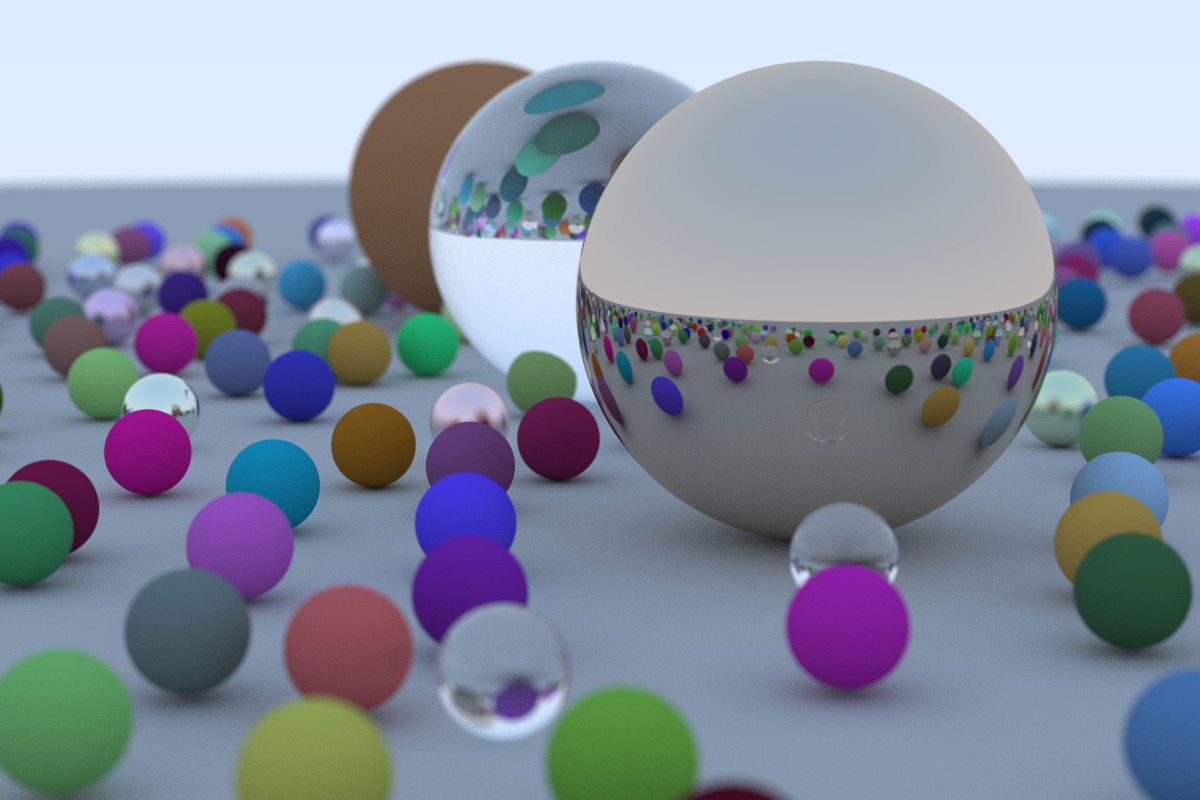
What started mainly as a toy project I wrote out of curiosity following the popular 'Ray Tracing in One Weekend' (RTOW) (Shirley 2020) book 5, anyhow made me appreciate the advantage of a generic raytracer (see fig. 1(a) for the final result of that book, created by this project). Generic meaning that the scene to be rendered is described by objects placed in simulated 3D world space. This reduces the amount of code that needs to be checked for correctness by orders of magnitude (reflection for one material type is a few line function, instead of having lines of code for every single reflection in a hardcoded raytracer). It also makes the program much more flexible to support different setups. In particular though, the concept of a camera independent of the scene geometry allows to visualize the scene (obviously the entire purpose of a normal raytracer!).
As a personal addition to the RTOW project, I implemented rendering to an SDL2 (Schmidt 2022b) window and handling mouse and keyboard inputs to produce an interactive real-time raytracer (this was early 2021). This sparked the idea to use the same approach for our axion raytracer. I pitched the idea to Johanna, but did not manage to convince her 6. While working on finalizing the axion image and X-ray finger simulations for this thesis, several big discrepancies between our raytracing results and those used for the CAST Nature paper in 2017 (Collaboration and others 2017) were noticed. The latter were done by Michael Pivovaroff at LLNL using a private in-house raytracer 7. The need to better verify the correctness of our own raytracing simulation lead me down the path of finishing the project of turning the RTOW based raytracer into an axion X-ray raytracer. This way verifying correctness was easier. Some additional features of the second book of the ROTW series were added (light sources among others) and other aspects were inspired by Physically Based Rendering (Pharr, Jakob, and Humphreys 2016) (in particular the idea of propagating multiple energies in each ray).
The result is TrAXer (Schmidt 2023), an interactive real-time visible
light and X-ray raytracer. In essence it is two raytracers in
one. First, a 'normal' visible light raytracer, which the camera
uses. Secondly, an X-ray raytracer. Both use the same raytracing
logic, but they differ in sampling. For visible light we emit rays
from the camera into the scene, while for X-rays we emit from an X-ray
source (an object placed in the scene, for example the Sun). Both of
these run in parallel. Scenes are defined by placing geometric
primitives with different materials (glass, metal etc.) into the
scene.
The X-ray raytracer is used by choosing X-ray emitting materials and adding another object as an X-ray target (another material), which the X-ray sampling will be biased towards. There is further a specific X-ray material an object can be made of, which behaves as expected when hit by an X-ray, calculated using (Schmidt and SciNim contributors 2022). Behavior is described by the reflectivity computed via the Fresnel equations as discussed in sec. 6.1.2. To simulate reflectivity of the LLNL telescope, the depth graded multilayers of the different layers are taken into account. X-ray transmission is currently not implemented, but only because there is no need for us. The addition would be easy based on mass attenuation coefficients and the Fresnel equations for transmission.
In order to detect and read out results from the X-ray raytracing, we place "image sensors" into the scene. They use a special material, which accumulates X-rays hitting them, split into spatial pixels. For visible light they simply emit the current values stored in each pixel of the image sensor, mapped to the Viridis color scale.
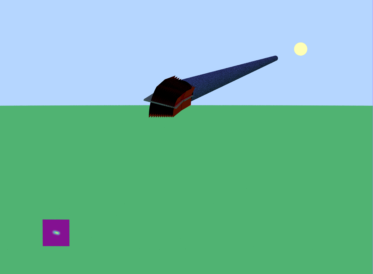
These things are visible in the example screenshot showing the "CAST" scene in fig. 1(b). The view is seen from behind and above the setup with a narrow field of view (like a telephoto lens). Only relevant pieces of the setup are placed into the scene (partially for performance, although bounding volume hierarchies help there, mostly for simplicity). The Sun is visible on the right side, emitting a yellow hue for the visible rays and an invisible X-ray spectrum following the expected solar axion flux (with correct radial emission). The long blueish tube is the inner bore of the CAST magnet. Then, with red hues (in visible light) we have the LLNL telescope. In the bottom left is the image sensor, which has the same physical size as the center GridPix of the Septemboard detector and is placed in the focal point of the telescope. As every object of the scene is floating above the earth, combined with the telephoto like view, the sensor looks a bit odd. 8
37.1.1. Discrepancies raytracer and LLNL raytracer extended
[ ]LINK TO DOCUMENT ANSWER TO IGOR! -> For that we need to host the document somewhere first!
37.1.2. Produce screenshots of TrAXer extended
This is simply a manual matter of running TrAXer with the desired
scene and taking screenshots manually. In theory we can save the frame
buffers using F5 and then produce an image from the raw data, but
there's not much point really.
The main question is what we really want to showcase.
For example to produce an example screenshot showcasing the original 'Raytracing in One Weekend' final image, we can do:
./raytracer --width 1200 --speed 10.0 --nJobs 32 --maxDepth 10 --spheres
and take a screenshot from:
Now looking at: (Point: [-4.278876423185614, 1.499472514352247, -5.283379080542512])
from : (Point: [-4.825481106391748, 1.938486638958975, -5.996463871218145]), yaw = 5.366388980384832, pitch = -0.4545011087932843
(we currently don't have a way to specify the starting location and point we look at. You see the current values printed to the terminal. Note that the movement speed can be adjusted using page up / page down).
[ ]Or use the original raytracing in one weekend screenshot we created? We are not using any depth of field in the current camera setup. -> I also get the impression that something about our image integration is not entirely working in the current raytracing code. The code has been running quite a while now (given that it's 28 threads), but the noise does not really get better. -> Well, our color code was simpler in the past. Just adding colors then dividing by num samples & gamma correcting. But it did not include yet how to integrate.
This way we took:
Let's place this screenshot next to one that showcases something more CAST related?
[ ]CAST screenshot. Maybe image sensor, magnet, telescope sun?
For example to simulate the 'realistic'
./raytracer \
    --width 1200 --speed 10.0 --nJobs 32 --vfov 15 --maxDepth 5 \
    --llnl --focalPoint --sourceKind skSun \
    --solarModelFile ~/CastData/ExternCode/AxionElectronLimit/resources/solar_model_dataframe.csv \
    --rayAt 1.0 \
    --sensorKind sSum \
    --usePerfectMirror=false \
    --ignoreWindow
from
[INFO] Current position (lookFrom) = (Point: [-207.533615402934, 75.77234678496751, -2003.522751711818]) at (lookAt) (Point: [-207.4532559830788, 75.71290478850352, -2002.527759745671])
37.2. A few more details about the LLNL telescope
The Lawrence Livermore National Laboratory, introduced in sec. 5.1.4, is the X-ray telescope of interest for us. Let us now first get an overview of the telescope and its construction itself, before we move on to comparing the TrAXer simulations with PANTER measurements and raytracing simulations from Michael Pivovaroff from LLNL.
Its design follows the technology developed for the NuSTAR mission (Harrison et al. 2013, 2006; Koglin et al. 2009; Craig et al. 2011; Hailey et al. 2010). This means it is not a true Wolter optic (meaning parabolic and hyperbolic mirrors), but instead uses a cone approximation (Petre and Serlemitsos 1985), which are easier to produce and in particular for CAST provide more than enough angular resolution.
It consists of two sets of 13 layers. Each mirror has a physical length of \(\SI{225}{mm}\) and thickness of \(d_{\text{glass}} = \SI{0.21}{mm}\). These mirrors are made of glass, which are thermally-formed ("slumped") into the conical shapes. Production of the mirrors happened at the National Space Institute at the Technical University of Denmark (DTU Space) as part of the PhD thesis of Anders Jakobsen (Jakobsen 2015). The first sets of layers \(i\) describe truncated coni with a remaining height of \(\SI{225}{mm}\), an arc angle of \(\SI{30}{°}\), a radius on the opening end 9 of \(R_{1,i}\) and a cone angle of \(α_i\). That is for each layer a non-truncated cone would have a total height of \(h = R_{1,i} / \tan{α_i}\). The second set of 13 layers only differs by their radii, \(R_{4,i}\) on the opening end and an angle of \(3 α_i\). In the horizontal direction along the optical axis of the telescope, there is a spacing of \(x_{\text{sep}} = \SI{4}{mm}\) between each set of layers. Due to the tilted angle the physical distance between each set is minutely larger. Combined the telescope thus has a length of roughly \(\SI{454}{mm}\).
One can define additional helpful radii, \(R_{2,i}\) the minimum radius of the first set of cones, \(R_{4,i}\) the maximum radii of the opening end of the second set of mirrors and finally \(R_{3,i}\), the radius at the mid point where the hypothetical extension of the first layer and last layer would touch at \(x = \SI{2}{mm}\) from each set of mirrors. Equations \eqref{eq:llnl_rest:radii_eqs} specify how these numbers are related with \(l\) the length of the mirrors.
\begin{align} \label{eq:llnl_rest:radii_eqs} R_{2,i} &= R_{3,i} + 0.5 x_{\text{sep}} \tan(α_i) \\ R_{1,i} &= R_{2,i} + l \sin(α_i) \\ R_{4,i} &= R_{3,i} - 0.5 x_{\text{sep}} \tan(3α_i) \\ R_{5,i} &= R_{4,i} - l \sin(3α_i) \end{align}which we can rewrite to compute everything from \(R_{1,i}\) by:
\begin{align*} R_{2,i} &= R_{1,i} - l \sin(α_i) \\ R_{3,i} &= R_{2,i} - 0.5 x_{\text{sep}} \tan(α_i) \\ R_{4,i} &= R_{3,i} - 0.5 x_{\text{sep}} \tan(3α_i) \\ R_{5,i} &= R_{4,i} - l \sin(3α_i) \end{align*}I emphasize this, because this conical nature describes the entire telescope as long as the radii \(R_{1,i}\), \(R_{4,i}\) and angle \(α_i\) are known. 10
Alternatively, this can also be used to construct an optimal conical telescope from a starting radius \(R_{1,0}\) (typically called the "mandrel"), if the iterative condition \(R_{3,i+1} = R_{1,i} + d_{\text{glass}}\) is employed (in this case some target parameters are needed of course, like focal length, \(x_{\text{sep}}\) and a few more).
To calculate the focal length \(f\) of an X-ray telescope of the Wolter type, we can use the Wolter equation,
\[ \tan(4α_i) = \frac{R_{3,i,\text{virtual}}}{f} \]
where \(α_i\) is the angle of the \(i^{\text{th}}\) layer and \(R_{3,i,\text{virtual}}\) is the radius corresponding to the virtual reflection point. Due to the double reflection inherent to a Wolter telescope, the incoming ray picks up a total angle of \(4α\) (\(0\) to \(2α\) after first reflection of the shell with angle \(α\), then \(2α\) to \(4α\) after reflecting from second shell of angle \(3α\)). The virtual radius is the radius at the point if one extends the incoming ray through the first set of mirrors and reflects at a single virtual mirror of an angle \(4α\) precisely at the midpoint of the telescope. This is illustrated in fig. 3, which is an adapted version of fig. 4.6 from A. Jakobsen's PhD thesis (Jakobsen 2015) to better illustrate this.
In addition to the PhD thesis mentioned, there is a paper (Aznar et al. 2015) about the telescope for CAST and initial results. Note though, that both the PhD thesis and the paper contain contradicting and wrong information about the details of the telescope design. Neither (nor combined do they) describe the real telescope. 11 , 12 Thanks to the help of and personal communication with Jaime Ruz and Julia Vogel we were able to both clear up confusions and find the original numbers of the telescope that were actually built. Table 37 gives an overview of the telescope design. It is adapted from (Aznar et al. 2015), but modified to use the correct numbers. Then in tab. 38 is the list of all layers and their corresponding radii in detail as given to me by Jaime Ruz.
| Property | Value |
|---|---|
| Mirror substrates | glass, Schott D263 |
| Substrate thickness | \(\SI{0.21}{mm}\) |
| \(l\), length of upper and lower mirrors | \(\SI{225}{mm}\) |
| Overall telescope length | \(\sim\SI{454}{mm}\) |
| \(f\) , focal length | \(\SI{1500}{mm}\) |
| Layers | 13 |
| Total number of individual mirrors in optic | 26 |
| \(R_{1,i}\) , range of maximum radii | \(\SIrange{63.24}{102.38}{mm}\) |
| \(R_{3,i}\) , range of mid-point radii | \(\SIrange{62.07}{100.5}{mm}\) |
| \(R_{5,i}\) , range of minimum radii | \(\SIrange{53.88}{87.19}{mm}\) |
| \(α\), range of graze angles | \(\SIrange{0.592}{0.958}{°}\) |
| Azimuthal extent | \(\sim\SI{30}{°}\) |
| i | \(R_1\) [\(\si{mm}\)] | \(R_2\) [\(\si{mm}\)] | \(R_3\) [\(\si{mm}\)] | \(R_4\) [\(\si{mm}\)] | \(R_5\) [\(\si{mm}\)] | α [\(\si{°}\)] | 3α [\(\si{°}\)] |
|---|---|---|---|---|---|---|---|
| 1 | 63.2384 | 60.9121 | 60.8914 | 60.8632 | 53.8823 | 0.5924 | 1.7780 |
| 2 | 65.8700 | 63.4470 | 63.4255 | 63.3197 | 56.0483 | 0.6170 | 1.8520 |
| 3 | 68.6059 | 66.0824 | 66.0600 | 65.9637 | 58.3908 | 0.6426 | 1.9288 |
| 4 | 71.4175 | 68.7898 | 68.7664 | 68.6794 | 60.7934 | 0.6692 | 2.0086 |
| 5 | 74.4006 | 71.6647 | 71.6404 | 71.5582 | 63.3473 | 0.6967 | 2.0913 |
| 6 | 77.4496 | 74.6014 | 74.5761 | 74.4997 | 65.9515 | 0.7253 | 2.1773 |
| 7 | 80.6099 | 77.6452 | 77.6188 | 77.5496 | 68.6513 | 0.7550 | 2.2665 |
| 8 | 83.9198 | 80.8341 | 80.8067 | 80.7305 | 71.4688 | 0.7858 | 2.3591 |
| 9 | 87.3402 | 84.1290 | 84.1005 | 84.0137 | 74.3748 | 0.8178 | 2.4553 |
| 10 | 90.8910 | 87.5495 | 87.5198 | 87.4316 | 77.4012 | 0.8510 | 2.5551 |
| 11 | 94.5780 | 91.1013 | 91.0704 | 90.9865 | 80.5497 | 0.8850 | 2.6587 |
| 12 | 98.3908 | 94.7737 | 94.7415 | 94.6549 | 83.7962 | 0.9211 | 2.7662 |
| 13 | 102.381 | 98.6187 | 98.5853 | 98.4879 | 87.1914 | 0.9581 | 2.8778 |

Having discussed the physical layout of the telescope, let us quickly talk about the telescope coatings. In contrast to telescope like the ABRIXAS or XMM-Newton optics, which use a single layer gold coating, the NuSTAR design uses a depth graded multilayer coating as introduced in sec. 6.1.2. There are four different 'recipes', used for different layers. All recipes are a depth graded multilayer of different number of Pt/C layers.
Note that in this terminology the high \(Z\) material (platinum) is actually below the low \(Z\) material (carbon) contrary to what Pt/C might imply!
Table 39 gives an overview of which recipes are used for which layer and how they differ. \(d_{\text{min}}\) is the minimum thickness of one multilayer and \(d_{\text{max}}\) the maximum thickness. The top most multilayer is the thickest. \(Γ\) is the ratio of the top to bottom material in each multilayer.
For example recipe 1 has a top multilayer of carbon of a thickness \(Γ · d_{\text{max}} = \SI{10.125}{nm}\) on top of \((1 - Γ) · d_{\text{max}} = \SI{12.375}{nm}\) of platinum. Because recipe 1 only has 2 such multilayers, the bottom Pt/C layer has a combined thickness of \(d_{\text{min}}\).
To reiterate the equations that describe the layer thicknesses for \(N\) layers as given in sec. 6.1.2, a depth-graded multilayer is described by the equation:
\begin{equation} \label{eq:appendix:depth_graded_multilayer} d_i = \frac{a}{(b + i)^c} \end{equation}where \(d_i\) is the depth of layer \(i\) (out of \(N\) layers),
\[ a = d_{\text{min}} (b + N)^c \]
and
\[ b = \frac{1 - N k}{k - 1} \]
with
\[ k = \left(\frac{d_{\text{min}}}{d_{\text{max}}}\right)^{\frac{1}{c}}. \]
In all four recipes used for the LLNL telescope the parameter \(c\) is set to 1.
| Recipe | # of layers | \(d_{\text{min}}\) [\(\si{nm}\)] | \(d_{\text{max}}\) [\(\si{nm}\)] | Γ |
|---|---|---|---|---|
| 1 | 2 | 11.5 | 22.5 | 0.45 |
| 2 | 4 | 7.0 | 19.0 | 0.45 |
| 3 | 4 | 5.5 | 16.0 | 0.4 |
| 4 | 2 | 5.0 | 14.0 | 0.4 |
Calculation of the reflectivity follows the equations also mentioned
in the theory section. The reflectivities of each layer are calculated
with (Schmidt and SciNim contributors 2022), which is used as part of the
material description in TrAXer.
37.2.1. Calculate angles and focal length based on Wolter equation for telescope data files extended
The following, initially adapted from ./../org/Mails/llnlAxionImage/llnl_axion_image.html and found in ./../org/Doc/LLNL_TrAXer_comparison/llnl_traxer_raytracing_comparison.html and ./../org/journal.html computes the expected focal length based on the Wolter equation:
\[ \tanh(4α) = \frac{R}{f} \]
where the radius \(R\) is the radius of the virtual reflection point of the combined telescope system.
The data files are ./../org/resources/LLNL_telescope/cast20l4_f1500mm_asBuilt.txt and ./../org/resources/LLNL_telescope/cast20l4_f1500mm_asDesigned.txt.
What we can see below is that the numbers from Anders' PhD thesis yield a telescope with focal length of \(\SI{1530}{mm}\) instead of the target. Also it computes the angles for all layers based on the radii.
The data file 'as built' is the one of main interest! The angles printed in the table below for that case are the ones shown in the main section above.
import math, sequtils, datamancer
const lMirror = 225.0
const xSep = 4.0

proc calcAngle(r1, r2: float): float =
  result = arcsin(abs(r1 - r2) / lMirror)

proc calcR3(r1, lMirror: float, α: float): float =
  let r2 = r1 - lMirror * sin(α)
  result = r2 - 0.5 * xSep * tan(α)

proc printTab(R1s, R2s, R4s, R5s: openArray[float]) =
  var df = newDataFrame()
  for i in 0 ..< R1s.len:
    let r1 = R1s[i]
    let r2 = R2s[i]
    let α = calcAngle(r1, r2)
    let r3 = calcR3(r1, lMirror, α)
    let r1minus = r1 - sin(α) * lMirror/2
    let fr3 = r3 / tan(4 * α)
    let fr1m = r1minus / tan(4 * α)
    df.add (i: i+1, f_R3: fr3.float, f_R1m: fr1m.float, α: α.radToDeg, R3: r3)
  echo df.toOrgTable

proc printBuiltTab(R1s, R2s, R4s, R5s: openArray[float]) =
  var df = newDataFrame()
  for i in 0 ..< R1s.len:
    let r1 = R1s[i]
    let r2 = R2s[i]
    let r4 = R4s[i]
    let r5 = R5s[i]
    let α = calcAngle(r1, r2)
    let α3 = calcAngle(r4, r5)
    let r3 = calcR3(r1, lMirror, α)
    df.add (i: i+1, R1: r1, R2: r2, R3: r3, R4: r4, R5: r5, α: α.radToDeg, α3: α3.radToDeg)
  echo df.rename(f{"3α" <- "α3"}).toOrgTable(precision = 6)

block AndersPhD:
  let R1s = @[63.006, 65.606, 68.305, 71.105, 74.011, 77.027, 80.157,
              83.405, 86.775, 90.272, 93.902, 97.668, 101.576, 105.632]
  let αs = @[0.579, 0.603, 0.628, 0.654, 0.680, 0.708, 0.737, 0.767,
             0.798, 0.830, 0.863, 0.898, 0.933, 0.970]
  proc calcR2(r1, α: float): float = r1 - sin(α.degToRad) * lMirror
  let R2s = toSeq(0 ..< R1s.len).mapIt(calcR2(R1s[it], αs[it]))
  echo "Using values from Anders PhD thesis"
  printTab(R1s, R2s, [], [])

block AsDesigned: # `cast20l4_f1500mm_asDesigned.txt`
  let R1s = [ 63.2412, 65.8741, 68.6075, 71.4450, 74.3908, 77.4488, 80.6233,
              83.9188, 87.3398, 90.8911, 94.5775, 98.4043, 102.377 ]
  let R2s = [ 60.9149, 63.4511, 66.0840, 68.8173, 71.6549, 74.6006, 77.6586,
              80.8331, 84.1286, 87.5496, 91.1008, 94.7872, 98.6139 ]
  let R4s = [ 60.8322, 63.3650, 65.9942, 68.7239, 71.5576, 74.4993, 77.5532,
              80.7234, 84.0144, 87.4307, 90.9771, 94.6586, 98.4801 ]
  let R5s = [ 53.8513, 56.0936, 58.4213, 60.8379, 63.3467, 65.9511, 68.6549,
              71.4617, 74.3755, 77.4003, 80.5403, 83.7999, 87.1836 ]
  let diffs = [ 10.3390, 10.7690, 11.2150, 11.6780, 12.1590, 12.6580, 13.1760,
                13.7130, 14.2710, 14.8500, 15.4510, 16.0740, 16.7210 ]
  echo "Using values from .txt file 'as designed'"
  printTab(R1s, R2s, R4s, R5s)

block AsBuilt: # `cast20l4_f1500mm_asBuilt.txt`
  # These are the numbers from the "as built" text file
  let R1s = [ 63.2384, 65.8700, 68.6059, 71.4175, 74.4006, 77.4496, 80.6099,
              83.9198, 87.3402, 90.8910, 94.5780, 98.3908, 102.381 ]
  let R2s = [ 60.9121, 63.4470, 66.0824, 68.7898, 71.6647, 74.6014, 77.6452,
              80.8341, 84.1290, 87.5495, 91.1013, 94.7737, 98.6187 ]
  let R4s = [ 60.8632, 63.3197, 65.9637, 68.6794, 71.5582, 74.4997, 77.5496,
              80.7305, 84.0137, 87.4316, 90.9865, 94.6549, 98.4879 ]
  let R5s = [ 53.8823, 56.0483, 58.3908, 60.7934, 63.3473, 65.9515, 68.6513,
              71.4688, 74.3748, 77.4012, 80.5497, 83.7962, 87.1914 ]
              # this last one should be the difference between R5 and R1
  let diffs = [ 10.339, 10.769, 11.216, 11.679, 12.160, 12.659, 13.176,
                13.714, 14.272, 14.851, 15.452, 16.076, 16.725  ]
  echo "Using values from .txt file 'as built'"
  printTab(R1s, R2s, R4s, R5s)

  # And now print the table to use in thesis
  echo "Overview of radii and angles of telescope was built:"
  printBuiltTab(R1s, R2s, R4s, R5s)
Using values from Anders PhD thesis
| i | fR3 | fR1m | α | R3 |
|---|---|---|---|---|
| 0 | 1501.1452 | 1529.7542 | 0.579 | 60.712099 |
| 1 | 1500.7995 | 1529.4071 | 0.603 | 63.217019 |
| 2 | 1500.2462 | 1528.8523 | 0.628 | 65.816977 |
| 3 | 1499.554 | 1528.1586 | 0.654 | 68.513974 |
| 4 | 1501.1365 | 1529.7394 | 0.68 | 71.316971 |
| 5 | 1500.4047 | 1529.0057 | 0.708 | 74.222046 |
| 6 | 1499.816 | 1528.4149 | 0.737 | 77.23716 |
| 7 | 1499.4292 | 1528.026 | 0.767 | 80.366313 |
| 8 | 1499.2931 | 1527.8876 | 0.798 | 83.613505 |
| 9 | 1499.4644 | 1528.0564 | 0.83 | 86.983737 |
| 10 | 1500.0058 | 1528.5952 | 0.863 | 90.483008 |
| 11 | 1499.1816 | 1527.768 | 0.898 | 94.110358 |
| 12 | 1500.579 | 1529.1623 | 0.933 | 97.879709 |
| 13 | 1500.8171 | 1529.397 | 0.97 | 101.78914 |
Using values from .txt file 'as designed'
| i | fR3 | fR1m | α | R3 |
|---|---|---|---|---|
| 0 | 1471.5582 | 1500.1664 | 0.59239799 | 60.894221 |
| 1 | 1471.5794 | 1500.1861 | 0.61702381 | 63.429561 |
| 2 | 1471.5244 | 1500.1297 | 0.64261747 | 66.061567 |
| 3 | 1471.5363 | 1500.1398 | 0.66915352 | 68.793941 |
| 4 | 1471.5242 | 1500.1259 | 0.69670838 | 71.630579 |
| 5 | 1471.5125 | 1500.1123 | 0.72530755 | 74.575281 |
| 6 | 1471.5293 | 1500.127 | 0.7549765 | 77.632245 |
| 7 | 1471.5027 | 1500.0982 | 0.78579169 | 80.805669 |
| 8 | 1471.5144 | 1500.1074 | 0.81775313 | 84.100053 |
| 9 | 1471.501 | 1500.0913 | 0.85093727 | 87.519895 |
| 10 | 1471.4966 | 1500.0841 | 0.88536962 | 91.069892 |
| 11 | 1471.453 | 1500.0374 | 0.92112663 | 94.755044 |
| 12 | 1471.2913 | 1499.8723 | 0.95831023 | 98.580446 |
Using values from .txt file 'as built'
| i | fR3 | fR1m | α | R3 |
|---|---|---|---|---|
| 0 | 1471.4905 | 1500.0987 | 0.59239799 | 60.891421 |
| 1 | 1471.4842 | 1500.091 | 0.61702381 | 63.425461 |
| 2 | 1471.4888 | 1500.094 | 0.64261747 | 66.059967 |
| 3 | 1470.948 | 1499.5516 | 0.66915352 | 68.766441 |
| 4 | 1471.7255 | 1500.3272 | 0.69670838 | 71.640379 |
| 5 | 1471.5282 | 1500.128 | 0.72530755 | 74.576081 |
| 6 | 1471.2753 | 1499.873 | 0.7549765 | 77.618845 |
| 7 | 1471.5209 | 1500.1164 | 0.78579169 | 80.806669 |
| 8 | 1471.5214 | 1500.1144 | 0.81775313 | 84.100453 |
| 9 | 1471.4993 | 1500.0896 | 0.85093727 | 87.519795 |
| 10 | 1471.5047 | 1500.0922 | 0.88536962 | 91.070392 |
| 11 | 1471.2434 | 1499.8278 | 0.92112663 | 94.741544 |
| 12 | 1471.6768 | 1500.2579 | 0.95810648 | 98.585253 |
Overview of radii and angles of telescope was built:
| i | R1 | R2 | R3 | R4 | R5 | α | 3α |
|---|---|---|---|---|---|---|---|
| 0 | 63.2384 | 60.9121 | 60.8914 | 60.8632 | 53.8823 | 0.592398 | 1.77796 |
| 1 | 65.87 | 63.447 | 63.4255 | 63.3197 | 56.0483 | 0.617024 | 1.85197 |
| 2 | 68.6059 | 66.0824 | 66.06 | 65.9637 | 58.3908 | 0.642617 | 1.92879 |
| 3 | 71.4175 | 68.7898 | 68.7664 | 68.6794 | 60.7934 | 0.669154 | 2.00856 |
| 4 | 74.4006 | 71.6647 | 71.6404 | 71.5582 | 63.3473 | 0.696708 | 2.09135 |
| 5 | 77.4496 | 74.6014 | 74.5761 | 74.4997 | 65.9515 | 0.725308 | 2.17731 |
| 6 | 80.6099 | 77.6452 | 77.6188 | 77.5496 | 68.6513 | 0.754977 | 2.26652 |
| 7 | 83.9198 | 80.8341 | 80.8067 | 80.7305 | 71.4688 | 0.785792 | 2.35914 |
| 8 | 87.3402 | 84.129 | 84.1005 | 84.0137 | 74.3748 | 0.817753 | 2.45528 |
| 9 | 90.891 | 87.5495 | 87.5198 | 87.4316 | 77.4012 | 0.850937 | 2.55507 |
| 10 | 94.578 | 91.1013 | 91.0704 | 90.9865 | 80.5497 | 0.88537 | 2.65866 |
| 11 | 98.3908 | 94.7737 | 94.7415 | 94.6549 | 83.7962 | 0.921127 | 2.76622 |
| 12 | 102.381 | 98.6187 | 98.5853 | 98.4879 | 87.1914 | 0.958106 | 2.87784 |
:shockedface: :explodinghead:
37.3. Comparison of TrAXer results with PANTER measurements
The LLNL telescope was tested and characterized at the PANTER X-ray test facility in
Munich in July 2016. It was reported on these tests during the
\(62^{\text{nd}}\) CAST collaboration meeting (CCM) on and
again in the CCM on . 13 These results are
valuable to us, because they can be used as a cross-check to verify
our TrAXer based raytracing simulations.
At the PANTER facility the X-ray source sits \(\SI{130.297}{m}\) away from the center of the telescope (the plane of the virtual reflection). It can be approximated as a source of radius \(\SI{0.42}{mm}\). The detector used to measure at PANTER is installed on the optical axis (i.e. directly 'in front of' the source). The telescope itself is offset by the radius of its shells, such that its optical axis aligns with the optical axis defined by the X-ray beam (instead of aligning the telescope entrance with the beam axis and the detector offset from it!). In this way the light entering the telescope does not enter perpendicular to the opening, but under an angle.
The setup of having such an effective point source implies that the best focal point will not be in the physical focal spot defined by the focal length, but slightly behind. At PANTER this was measured to be at \(\SI{1519}{mm}\) instead of \(\SI{1500}{mm}\) and provides a first check of our raytracer. When reproducing the same setup in TrAXer we find the smallest, most symmetric spot around the \(\SIrange{1519}{1520}{mm}\) mark as well. 14
In this setup three different X-ray fluorescence lines were measured. \(\ce{Al}\) Kα (\(\SI{1.49}{keV}\)), \(\ce{Ti}\) Kα (\(\SI{4.51}{keV}\)) and \(\ce{Fe}\) Kα (\(\SI{6.41}{keV}\)). We can compare the images between measurements and simulations as well as compute the 'half power diameter' (HPD). The HPD is the radius around the image center (based on the weighted mean center) in which \(\SI{50}{\%}\) of the flux is contained. This is computed based on the encircled energy function (EEF): integrate the flux in radial slices around the center, compute a radial cumulative distribution function and find the radius corresponding to \(\SI{50}{\%}\).
Let's consider the aluminum Kα lines. Fig. 4 compares the PANTER data, with the LLNL raytracing result and our raytracing result. 15 All three plots show the inner \(\num{3}·\SI{3}{mm²}\) of the image. Generally, the agreement is very good. The "bow tie" shape can be seen in all three figures.


Computing the encircled energy function yields a figure as shown in fig. 5. We see the HPD shown as the red line at a radius of \(r_{\text{HPD}} \approx \SI{0.79}{mm}\). This is converted to an HPD in arc seconds via
\[ α_{\text{HPD}} = \arctan\left( \frac{r_{\text{HPD}}}{f} \right) \]
where \(f\) is the focal length of the optic. This leads to an HPD of \(\SI{216.38}{\arcsecond}\), which is slightly above both the LLNL raytracing simulation (PANTER model) and the PANTER data. Doing this for all three fluorescence lines, we get the numbers shown in tab. 40, where the differences are even smaller. Therefore, our implementation of the raytracer including figure errors yields very compatible results to the LLNL model developed for PANTER. The usage of TrAXer as the tool of choice for the calculation of the axion image seems justified.
See sec. 37.3.1 below for more details on how the figure error is introduced and its parameters determined.

| Al Kα (1.49 keV) | |||
|---|---|---|---|
| 50% (HPD) | 80% circle | 90% circle | |
| Point source (perfect mirrors) | 168 arcsec | 270 arcsec | 313 arcsec |
| Point source (figure errors) | 206 | 387 | 568 |
| PANTER data | 206 | 397 | 549 |
| PANTER model | 211 | 391 | 559 |
| TrAXer (perfect mirrors) | 183.19 | 304.61 | 351.54 |
| TrAXer (figure errors) | 216.38 | 389.72 | 559.79 |
| Ti Kα (4.51 keV) | |||
| 50% (HPD) | 80% circle | 90% circle | |
| Point source (perfect mirrors) | 161 | 259 | 301 |
| Point source (figure errors) | 202 | 382 | 566 |
| PANTER data | 196 | 380 | 511 |
| PANTER model | 206 | 380 | 559 |
| TrAXer (perfect mirrors) | 174.84 | 288.54 | 333.75 |
| TrAXer (figure errors) | 207.43 | 378.16 | 552.55 |
| Fe Kα (6.41 keV) | |||
| 50% (HPD) | 80% circle | 90% circle | |
| Point source (perfect mirrors) | 144 | 233 | 265 |
| Point source (figure errors) | 184 | 350 | 541 |
| PANTER data | 196 | 364 | 483 |
| PANTER model | 185 | 348 | 516 |
| TrAXer (perfect mirrors) | 160.38 | 257.79 | 296.79 |
| TrAXer (figure errors) | 189.75 | 345.20 | 518.51 |
37.3.1. Definition of the figure error and parameter determination
The figure error implementation has multiple free parameters. Generally speaking upon reflection on a mirror surface, the reflected direction is slightly modified. Let \(\vec{r}_i\) be the incoming ray, \(\vec{n}\) the surface normal on which the ray reflects and \(\vec{r}_r\) the reflected ray. Reflection happens in the plane defined by \(\vec{n}\) and \(\vec{r}_{i,r}\). For a realistic figure error we wish to mainly vary the reflected direction in this plane around \(\vec{r}_r\), but still allow for smaller amounts in directions orthogonal. The vector orthogonal to this plane is
\[ \vec{n}_{\perp} = \vec{n} \times \vec{r}_r. \]
This orthogonal vector \(\vec{n}_{\perp}\) allow us further to construct a vector that is orthogonal to \(\vec{r}_r\) but in the plane of the incoming and outgoing ray,
\[ \vec{s} = \vec{n}_{\perp} \times \vec{r}_r. \]
Based on two fuzzing parameters \(f_{\parallel}\) and \(f_{\perp}\) we can then define the real reflected ray to be:
\[ \vec{r}_{\text{fuzzed}} = \vec{p}_{\text{hit}} + \vec{r}_r + f_{\parallel} · \vec{s} + f_{\perp} · \vec{n}_{\perp} \]
where \(\vec{p}_{\text{hit}}\) is the point at which the ray hit a mirror shell. Generally \(f_{\parallel}\) and \(f_{\perp}\) are parameters sampled from a normal distribution. In practice only \(f_{\perp}\) is directly sampled from a single normal distribution, while \(f_{\parallel}\) is – effectively – a mix of a narrow and a wide normal distribution. In total there are \(\num{5}\) input parameters, which define the final figure error model.
In order to find the best matching parameters, we perform non-linear optimization using a global derivative-free algorithm 16. This optimization calls the raytracer with a set of parameters in batch mode 17 up to a fixed set of rays, computes the HPD and radii containing \(\SI{80}{\%}\) and \(\SI{90}{\%}\) of the flux and finally computes the mean squared error of the target parameters given and the current values.
Ideally of course, one would use a map of the real surface roughness
of each mirror shell (as done in (Brejnholt 2012) for the NuSTAR
telescope using MT_RAYOR) and use that as the basis for more
accurate reflection on the surface.
See fig. 6 for a comparison of the image without any figure error (assuming perfect mirrors) and the final figure errors (which are the ones used in the table and plots of the previous section). The right plot shows the same data as seen in fig. 4(c) above. The difference is massive in the sharpness of the data.


37.3.1.1. Determining the optimal parameters extended
The optimal parameters that we use nowadays, are determined by starting with the Al Kα line.
The program performing the optimization is optimize_figure_error.nim
in the TrAXer repository (Schmidt 2023).
./optimize_figure_error \
    --hpd 206 --c80 397 --c90 568 \
    --bufOutdir out_GN_DIRECT_L \
    --shmFile /dev/shm/image_sensor_GN_DIRECT_L.dat
which calls the raytracer with a set of fuzzing parameters, computes the EEF for the HPD, c80 and c90 radii and comparing them to the given arguments (these are the target values for the PANTER data of the Al Kα line, see tab. 40).
See the NLopt documentation about the algorithm here: https://nlopt.readthedocs.io/en/latest/NLopt_Algorithms/#direct-and-direct-l
To run the program you need to first compile the raytracer,
nim c -d:ThreadPoolSize=32 -d:danger raytracer.nim
and the calc_eef helper:
nim c -d:danger calc_eef.nim
after checking out the repository.
37.3.2. More notes extended
See the following documents for more information about the LLNL
telescope and the raytracer. It includes a lot of understanding
various confusions mentioned above (and more), the reasoning as to how
I ended up finishing TrAXer in the first place (reply to Igor),
development notes of it and further questions and finally lots more
about these PANTER / TrAXer comparisons.
- ./../org/Doc/LLNL_def_REST_format/llnl_def_rest_format.html
- ./../org/Mails/igorReplyLLNL/igor_reply_llnl_axion_image.html
 -> These are part of
./../org/Doc/StatusAndProgress.html!
-> These are part of
./../org/Doc/StatusAndProgress.html!- ./../org/Mails/llnlAxionImage/llnl_axion_image.html
- ./../org/Doc/LLNL_TrAXer_comparison/llnl_traxer_raytracing_comparison.html
37.3.3. Half-power diameter definition / calculation extended
The slides from the \(62^{\text{nd}}\) CCM contain the following explanation about how the HPD should be calculated on slide 10:
- Actually, more useful to consider the encircled energy function (EEF)
- Draw a circle around the PSF, integrate the flux, record the value
- Repeat process, building up cumulative distribution as a function of radius; normalize to unity
- It’s the integral of the PSF
- The half-power diameter (HPD) is just diameter where the EEF = 50%
The slide in the CCM from Jan 2017 showing their EEFs is slide 17, fig. 7.

37.3.4. Comparison of slices along short axis extended
The CCM presentation from Jan 2017 contains also plots that sum the signal along each axis in the data. These can be used for a more precise determination of whether our signal is too wide (due to too large figure error) or not.
See slide 12,
 ,
,
namely the plot in the bottom right. It is quite hard to get precise numbers from it, but the 50% amplitude is roughly near the \(\SI{0.1}{mm}\) mark. Reproducing a similar plot with our data, yields fig. 8. We see that the \(\SI{50}{\%}\) mark here is at \(\SI{0.13}{mm}\). Maybe this is a slight indication for a somewhat too wide result. But well. The actual problem with the HPD as mentioned in the main text still remains.

37.3.5. More on figure errors extended
One of the main issues with figure errors – aside from not being very well defined – is that they are usually quoted as a number for the entire X-ray optic. This is problematic when implementing it in a raytracer however, because the figure error is a property of the material surface. And because an X-ray optic works by a double reflection, the uncertainty is squared (in a non-trivial way). Therefore, it is not straightforward to simply compute a correct number to apply to the uncertainty of the scattering on the mirror surfaces from a real measurement.
(Hey, if you do know how to do it, let me know!)
37.3.6. Produce \(\ce{Al}Kα\) plot from TrAXer data extended
(We define a simple helper script to extract the last bits of output from the raytracing program
import strutils
for l in data.len - lines ..< data.len:
  echo data[l].join(" ")
)
In order to generate the data file needed for the HPD calculation and
plot used above, we need to first run the raytracer to produce the
binary data files and then use plotBinary to produce the
plots. Let's produce all three targets now.
The HPD values are extracted from the output of plotBinary or from
the *_hpd_via_eef.pdf plot annotations.
37.3.6.1. Al Kα
Run the raytracer, note the energyMin and energyMax.
./raytracer \
    --width 1200 --speed 10.0 --nJobs 32 --vfov 45 --maxDepth 10 \
    --llnl --focalPoint \
    --sourceKind skXrayFinger \
    --rayAt 1.013 \
    --sensorKind sSum \
    --energyMin 1.48 --energyMax 1.50 \
    --usePerfectMirror=false \
    --ignoreWindow \
    --sourceDistance 130.297.m \
    --sourceRadius 0.42.mm \
    --telescopeRotation 90.0 \
    --sourceOnOpticalAxis \
    --ignoreMagnet \
    --targetRadius 40.mm
[INFO] Writing buffers to binary files. [INFO] Writing file: out/buffer2023-11-12T12:56:26+01:00typeuint32len1440000width1200height1200.dat [INFO] Writing file: out/counts2023-11-12T12:56:26+01:00typeintlen1440000width1200height1200.dat [INFO] Writing file: out/imagesensor02023-11-12T12:56:26+01:00_dx14.0dy14.0dz0.1typefloatlen1000000width1000height1000.dat
Once you deem that enough statistics has been accumulated, press F5
on your keyboard to save all buffers to binary files. The output
filenames will be printed to the terminal.
And then with the produced binary files we can plot them and compute
the HPDs (note: we produce it such that text matches for the 3 plots
side by side and then with F_WIDTH=0.9 for the HPD plot and with
F_WIDTH=0.5 for the perfect/imperfect comparison):
F_WIDTH=0.3333333 USE_TEX=true ./plotBinary \
    --dtype float \
    -f out/image_sensor_0_2023-11-12T12:56:26+01:00__dx_14.0_dy_14.0_dz_0.1_type_float_len_1000000_width_1000_height_1000.dat \
    --invertY \
    --out ~/phd/Figs/raytracing/llnlPanter/panter_source_Al_Kalpha_imperfect_mirrors_3x3mm_fWidth0.3.pdf \
    --inPixels=false \
    --title "Al Kα, 1.49 keV, 3x3 mm, figure errors, source optical axis" \
    --xrange 1.5
F_WIDTH=0.5 USE_TEX=true ./plotBinary \
    --dtype float \
    -f out/image_sensor_0_2023-11-12T12:56:26+01:00__dx_14.0_dy_14.0_dz_0.1_type_float_len_1000000_width_1000_height_1000.dat \
    --invertY \
    --out ~/phd/Figs/raytracing/llnlPanter/panter_source_Al_Kalpha_imperfect_mirrors_3x3mm_fWidth0.5.pdf \
    --inPixels=false \
    --title "Al Kα, 1.49 keV, 3x3 mm, figure errors, source optical axis" \
    --xrange 1.5
USE_TEX=true ./plotBinary \
    --dtype float \
    -f out/image_sensor_0_2023-11-12T12:56:26+01:00__dx_14.0_dy_14.0_dz_0.1_type_float_len_1000000_width_1000_height_1000.dat \
    --invertY \
    --out ~/phd/Figs/raytracing/llnlPanter/panter_source_Al_Kalpha_imperfect_mirrors_3x3mm.pdf \
    --inPixels=false \
    --title "Al Kα, 1.49 keV, 3x3 mm, figure errors, source optical axis" \
    --xrange 1.5


- Perfect mirrors
Perfect mirror:
./raytracer \
    --width 1200 --speed 10.0 --nJobs 32 --vfov 45 --maxDepth 10 \
    --llnl --focalPoint \
    --sourceKind skXrayFinger \
    --rayAt 1.013 \
    --sensorKind sSum \
    --energyMin 1.48 --energyMax 1.49 \
    --usePerfectMirror=true \
    --ignoreWindow \
    --sourceDistance 130.297.m \
    --sourceRadius 0.42.mm \
    --telescopeRotation 90.0 \
    --sourceOnOpticalAxis \
    --ignoreMagnet \
    --targetRadius 40.mm
[INFO] Writing buffers to binary files. [INFO] Writing file: out/buffer2023-11-11T09:31:09+01:00typeuint32len1440000width1200height1200.dat [INFO] Writing file: out/counts2023-11-11T09:31:09+01:00typeintlen1440000width1200height1200.dat [INFO] Writing file: out/imagesensor02023-11-11T09:31:09+01:00_dx14.0dy14.0dz0.1typefloatlen1000000width1000height1000.dat
Create the plots (only in 3x3 mm):
F_WIDTH=0.5 USE_TEX=true ./plotBinary \
    --dtype float \
    -f out/image_sensor_0_2023-11-11T09:31:09+01:00__dx_14.0_dy_14.0_dz_0.1_type_float_len_1000000_width_1000_height_1000.dat \
    --invertY \
    --out ~/phd/Figs/raytracing/llnlPanter/panter_source_Al_Kalpha_perfect_mirrors_3x3mm_fWidth0.5.pdf \
    --inPixels=false \
    --title "Al Kα, 1.49 keV, 3x3 mm, source optical axis" \
    --xrange 1.5
Produces the following figures:

Figure 14: Figure 212: Our result Al Kα as 3x3 mm with perfect mirrors 
Figure 15: Figure 213: Our result Al Kα as 3x3 mm with perfect mirrors, log10 
Figure 16: Figure 214: HPD in X for perfect mirrors of Al Kα 
Figure 17: Figure 215: HPD in Y for perfect mirrors of Al Kα 
Figure 18: Figure 216: HPD of Al Kα computed from the EEF (radial cumulative distribution function, encircled energy)
37.3.6.2. Ti Kα
Run the raytracer, note the energyMin and energyMax.
./raytracer \
    --width 1200 --speed 10.0 --nJobs 32 --vfov 45 --maxDepth 10 \
    --llnl --focalPoint \
    --sourceKind skXrayFinger \
    --rayAt 1.013 \
    --sensorKind sSum \
    --energyMin 4.50 --energyMax 4.52 \
    --usePerfectMirror=false \
    --ignoreWindow \
    --sourceDistance 130.297.m \
    --sourceRadius 0.42.mm \
    --telescopeRotation 90.0 \
    --sourceOnOpticalAxis \
    --ignoreMagnet \
    --targetRadius 40.mm
[INFO] Writing buffers to binary files. [INFO] Writing file: out/buffer2023-11-12T12:58:39+01:00typeuint32len1440000width1200height1200.dat [INFO] Writing file: out/counts2023-11-12T12:58:39+01:00typeintlen1440000width1200height1200.dat [INFO] Writing file: out/imagesensor02023-11-12T12:58:39+01:00_dx14.0dy14.0dz0.1typefloatlen1000000width1000height1000.dat
./plotBinary \
    --dtype float \
    -f out/image_sensor_0_2023-11-12T12:58:39+01:00__dx_14.0_dy_14.0_dz_0.1_type_float_len_1000000_width_1000_height_1000.dat \
    --invertY \
    --out ~/phd/Figs/raytracing/llnlPanter/panter_source_Ti_Kalpha_imperfect_mirrors_3x3mm.pdf \
    --inPixels=false \
    --title "Ti Kα, 4.51 keV, 3x3 mm, figure errors, source optical axis" \
    --xrange 1.5


- Perfect mirrors
Perfect mirror:
./raytracer \
    --width 1200 --speed 10.0 --nJobs 32 --vfov 45 --maxDepth 10 \
    --llnl --focalPoint \
    --sourceKind skXrayFinger \
    --rayAt 1.013 \
    --sensorKind sSum \
    --energyMin 4.50 --energyMax 4.52 \
    --usePerfectMirror=true \
    --ignoreWindow \
    --sourceDistance 130.297.m \
    --sourceRadius 0.42.mm \
    --telescopeRotation 90.0 \
    --sourceOnOpticalAxis \
    --ignoreMagnet \
    --targetRadius 40.mm
[INFO] Writing buffers to binary files. [INFO] Writing file: out/buffer2023-11-11T09:37:15+01:00typeuint32len1440000width1200height1200.dat [INFO] Writing file: out/counts2023-11-11T09:37:15+01:00typeintlen1440000width1200height1200.dat [INFO] Writing file: out/imagesensor02023-11-11T09:37:15+01:00_dx14.0dy14.0dz0.1typefloatlen1000000width1000height1000.dat
./plotBinary \
    --dtype float \
    -f out/image_sensor_0_2023-11-11T09:37:15+01:00__dx_14.0_dy_14.0_dz_0.1_type_float_len_1000000_width_1000_height_1000.dat \
    --invertY \
    --out ~/phd/Figs/raytracing/llnlPanter/panter_source_Ti_Kalpha_perfect_mirrors_3x3mm.pdf \
    --inPixels=false \
    --title "Ti Kα, 4.51 keV, 3x3 mm, source optical axis" \
    --xrange 1.5

Figure 24: Figure 222: Our result Ti Kα as 3x3 mm with perfect mirrors 
Figure 25: Figure 223: Our result Ti Kα as 3x3 mm with perfect mirrors, log10 
Figure 26: Figure 224: HPD in X for perfect mirrors of Ti Kα 
Figure 27: Figure 225: HPD in Y for perfect mirrors of Ti Kα 
Figure 28: Figure 226: HPD of Ti Kα computed from the EEF (radial cumulative distribution function, encircled energy)
37.3.6.3. Fe Kα
Run the raytracer, note the energyMin and energyMax.
./raytracer \
    --width 1200 --speed 10.0 --nJobs 32 --vfov 45 --maxDepth 10 \
    --llnl --focalPoint \
    --sourceKind skXrayFinger \
    --rayAt 1.013 \
    --sensorKind sSum \
    --energyMin 6.39 --energyMax 6.41 \
    --usePerfectMirror=false \
    --ignoreWindow \
    --sourceDistance 130.297.m \
    --sourceRadius 0.42.mm \
    --telescopeRotation 90.0 \
    --sourceOnOpticalAxis \
    --ignoreMagnet \
    --targetRadius 40.mm
[INFO] Writing buffers to binary files. [INFO] Writing file: out/buffer2023-11-12T12:59:52+01:00typeuint32len1440000width1200height1200.dat [INFO] Writing file: out/counts2023-11-12T12:59:52+01:00typeintlen1440000width1200height1200.dat [INFO] Writing file: out/imagesensor02023-11-12T12:59:52+01:00_dx14.0dy14.0dz0.1typefloatlen1000000width1000height1000.dat
./plotBinary \
    --dtype float \
    -f out/image_sensor_0_2023-11-12T12:59:52+01:00__dx_14.0_dy_14.0_dz_0.1_type_float_len_1000000_width_1000_height_1000.dat \
    --invertY \
    --out ~/phd/Figs/raytracing/llnlPanter/panter_source_Fe_Kalpha_imperfect_mirrors_3x3mm.pdf \
    --inPixels=false \
    --title "Fe Kα, 6.41 keV, 3x3 mm, figure errors, source optical axis" \
    --xrange 1.5


- Perfect mirrors
Perfect mirror:
./raytracer \
    --width 1200 --speed 10.0 --nJobs 32 --vfov 45 --maxDepth 10 \
    --llnl --focalPoint \
    --sourceKind skXrayFinger \
    --rayAt 1.013 \
    --sensorKind sSum \
    --energyMin 6.39 --energyMax 6.41 \
    --usePerfectMirror=true \
    --ignoreWindow \
    --sourceDistance 130.297.m \
    --sourceRadius 0.42.mm \
    --telescopeRotation 90.0 \
    --sourceOnOpticalAxis \
    --ignoreMagnet \
    --targetRadius 40.mm
[INFO] Writing buffers to binary files. [INFO] Writing file: out/buffer2023-11-11T09:41:47+01:00typeuint32len1440000width1200height1200.dat [INFO] Writing file: out/counts2023-11-11T09:41:47+01:00typeintlen1440000width1200height1200.dat [INFO] Writing file: out/imagesensor02023-11-11T09:41:47+01:00_dx14.0dy14.0dz0.1typefloatlen1000000width1000height1000.dat
./plotBinary \
    --dtype float \
    -f out/image_sensor_0_2023-11-11T09:41:47+01:00__dx_14.0_dy_14.0_dz_0.1_type_float_len_1000000_width_1000_height_1000.dat \
    --invertY \
    --out ~/phd/Figs/raytracing/llnlPanter/panter_source_Fe_Kalpha_perfect_mirrors_3x3mm.pdf \
    --inPixels=false \
    --title "Fe Kα, 6.41 keV, 3x3 mm, source optical axis" \
    --xrange 1.5

Figure 34: Figure 232: Our result Fe Kα as 3x3 mm with perfect mirrors 
Figure 35: Figure 233: Our result Fe Kα as 3x3 mm with perfect mirrors, log10 
Figure 36: Figure 234: HPD in X for perfect mirrors of Fe Kα 
Figure 37: Figure 235: HPD in Y for perfect mirrors of Fe Kα 
Figure 38: Figure 236: HPD of Fe Kα computed from the EEF (radial cumulative distribution function, encircled energy)
37.4. Computing an axion image with TrAXer
The previous section provides us with reasonable guarantees that our raytracer produces compatible results to PANTER measurements and the LLNL raytracing results. In particular for the axion-electron coupling we do not wish to reuse the raytracing prediction for the solar axion image computed by Michael Pivovaroff at LLNL, as used in the CAST Nature 2017 paper (Collaboration and others 2017) paper. 18 This is because of the different radial emission profile (compare fig. #fig:theory:solar_axion_flux:radial_dependence_ksvz_dfsz). And for the chameleon, due to its production in the solar tachocline, this is of course absolutely mandatory.
To simulate the solar axion image, we use the scene already shown in fig. 1(b). The Sun is placed as an X-ray emitter 19 at \(\SI{0.989}{AU}\) away 20 from the telescope. It emits X-rays of energies and from radii corresponding to the distribution seen in fig. #fig:theory:solar_axion_flux:flux_vs_energy_and_radius calculated using the opacity calculation code (Von Oy 2023) also developed by Johanna von Oy during her master thesis (Von Oy 2020). The calculations are based on the AGSS09 solar model (Asplund et al. 2009; Serenelli et al. 2009). The telescope is rotated under the angle it was installed at CAST, as deduced from the X-ray finger taken at CAST, fig. #fig:cast:xray_finger_centers (about \(\SI{14}{°}\)). The image sensor is placed slightly in front of the focal point. \(\SI{1492.93}{mm}\) away from the center of the telescope (to the virtual reflection point) instead of \(\SI{1500}{mm}\) to account for the median conversion point of the X-rays of the expected axion electron X-ray flux (as mentioned in sec. 13.10.5 and calculated in 36).
With all these in place, the axion image comes out as seen in fig. 39(a). In comparison fig. 39(b) shows the axion image as computed by the LLNL raytracing code (albeit only for the axion-photon coupling and related emission). The similarity between the two images is implying our raytracing simulation is sensible. Small differences are expected, not only because of a different solar emission. The different rotation angle is due to a different assumed rotation of the telescope. Our raytracing image shows a larger bulge in the center at very low intensity. The absolute size of the major flux region is very comparable. The slight asymmetry in our image is due to it being effectively \(\SI{8}{mm}\) in front of the focal point.


37.4.1. Further thoughts on the (missing?) bow tie extended
The bow tie feature in the raytracing images is partially present even in the perfect mirror raytracing results. But in those there is a hard cutoff at some point, because the last shell and largest angles have been reached. Once figure errors are included this turns into a much smoother process, resulting in the bow tie shape.
37.4.2. Note on conversion point extended
The calculation for the conversion point was mentioned in
[ ]REFERENCE
37.4.3. Generate solar axion image using TrAXer [/] extended
[X]WE FORGOT TO USE THE CORRECT DISTANCE, I.E. MEAN CONVERSION! -> Corrected.
The main ingredient we need to simulate the correct axion image is the data file that describes the radial and spectral emission of axions from the Sun.
Make sure to get the (Von Oy 2023) code:
cd <path/of/choice>
git clone https://github.com/jovoy/AxionElectronLimit.git
cd AxionElectronLimit
cd src
nim c -d:danger readOpacityFile
Note that you also need to download the OPCD files from the opacity
project https://cdsweb.u-strasbg.fr/topbase/TheOP.html.
Download the .tar file and place it in a location of your
choice. With that done, update the AxionElectronLimit config file
found in
./../CastData/ExternCode/AxionElectronLimit/config/config.toml
by setting the
opcdPath = "/home/basti/CastData/data/"
field under [ReadOpacityFile] to the correct directory. The
directory should point to the parent directory of the OPCD_3.3 dir.
If you do not have a config.toml file, just create a copy of the
config_default.toml as config.toml.
Now we can run readOpacityFile:
./readOpacityFile \
    --suffix "_0.989AU" \
    --distanceSunEarth 0.9891144450781392.AU \
    --fluxKind fkAxionElectronPhoton \
    --plotPath ~/phd/Figs/readOpacityFile/ \
    --outpath ~/phd/resources/readOpacityFile/
where we insert the correct distance from Sun to Earth, see sec. 13.10.2.1. And we set the fluxes to only those interactions we are interested in (ignoring things like plasmon interactions).
The output data will be written as a CSV file to a location also defined in the config file.
Using this CSV file, which should be called
solar_model_dataframe_fluxKind_fkAxionElectronPhoton_0.989AU.csv we
can run the raytracer, in this case in the focal point:
./raytracer \
    --width 1200 --speed 10.0 --nJobs 32 --vfov 15 --maxDepth 5 \
    --llnl --focalPoint --sourceKind skSun \
    --solarModelFile ~/CastData/ExternCode/AxionElectronLimit/resources/solar_model_dataframe_fluxKind_fkAxionElectronPhoton_0.989AU.csv \
    --sensorKind sSum \
    --usePerfectMirror=false \
    --ignoreWindow
[INFO] Writing buffers to binary files. [INFO] Writing file: out/buffer2023-11-12T16:12:11+01:00typeuint32len1440000width1200height1200.dat [INFO] Writing file: out/counts2023-11-12T16:12:11+01:00typeintlen1440000width1200height1200.dat [INFO] Writing file: out/imagesensor02023-11-12T16:12:11+01:00_dx14.0dy14.0dz0.1typefloatlen1000000width1000height1000.dat
[INFO] Writing buffers to binary files. [INFO] Writing file: out/buffer2023-11-10T12:40:44+01:00typeuint32len1440000width1200height1200.dat [INFO] Writing file: out/counts2023-11-10T12:40:44+01:00typeintlen1440000width1200height1200.dat [INFO] Writing file: out/imagesensor02023-11-10T12:40:44+01:00_dx14.0dy14.0dz0.1typefloatlen1000000width1000height1000.dat
The important point is the solarModelFile parameter and
--sensorKind sSum, which sets image sensors up to sum up all flux
contributions in each pixel (instead of just counting how many rays
hit each pixel). We do not want to have the GridPix window strongback
in the result.
It will sample in an energy range between 0.03 and 15 keV. The lower bound is due to the limit on the reflectivity calculation that is possible based on the atomic scattering factors.
Time to produce a plot of the image:
./plotBinary \
    --dtype float \
    -f out/image_sensor_0_2023-11-10T12:40:44+01:00__dx_14.0_dy_14.0_dz_0.1_type_float_len_1000000_width_1000_height_1000.dat \
    --invertY \
    --out ~/phd/Figs/raytracing/solar_axion_image_fkAxionElectronPhoton_0.989AU_old_figure_errors.pdf \
    --inPixels=false \
    --title "Solar axion image at 0.989 AU from Sun (old figure errors)"
With the new fuzzing logic:
./plotBinary \
    --dtype float \
    -f out/image_sensor_0_2023-11-12T16:12:11+01:00__dx_14.0_dy_14.0_dz_0.1_type_float_len_1000000_width_1000_height_1000.dat \
    --invertY \
    --out ~/phd/Figs/raytracing/solar_axion_image_fkAxionElectronPhoton_0.989AU.pdf \
    --inPixels=false \
    --title "Solar axion image at 0.989 AU from Sun (imperfect mirrors)"
For comparison let's also run the code without any figure errors:
./raytracer \
    --width 1200 --speed 10.0 --nJobs 32 --vfov 15 --maxDepth 5 \
    --llnl --focalPoint --sourceKind skSun \
    --solarModelFile ~/CastData/ExternCode/AxionElectronLimit/resources/solar_model_dataframe_fluxKind_fkAxionElectronPhoton_0.989AU.csv \
    --sensorKind sSum \
    --usePerfectMirror=true \
    --ignoreWindow
[INFO] Writing buffers to binary files. [INFO] Writing file: out/buffer2023-11-10T12:45:29+01:00typeuint32len1440000width1200height1200.dat [INFO] Writing file: out/counts2023-11-10T12:45:29+01:00typeintlen1440000width1200height1200.dat [INFO] Writing file: out/imagesensor02023-11-10T12:45:29+01:00_dx14.0dy14.0dz0.1typefloatlen1000000width1000height1000.dat
./plotBinary \
    --dtype float \
    -f out/image_sensor_0_2023-11-10T12:45:29+01:00__dx_14.0_dy_14.0_dz_0.1_type_float_len_1000000_width_1000_height_1000.dat \
    --invertY \
    --out ~/phd/Figs/raytracing/solar_axion_image_perfect_mirrors_fkAxionElectronPhoton_0.989AU.pdf \
    --inPixels=false \
    --title "Solar axion image at 0.989 AU from Sun, perfect mirrors"
And finally we also compute the axion image at the point of most
likely conversion of X-rays, i.e. at \(\SI{1492.93}{mm}\) instead of
\(\SI{1500}{mm}\). Thus, --rayAt 0.995286666667 (1492.93 / 1500) to
get the correct placement:
./raytracer \
    --width 1200 --speed 10.0 --nJobs 32 --vfov 15 --maxDepth 5 \
    --llnl --focalPoint --sourceKind skSun \
    --solarModelFile ~/CastData/ExternCode/AxionElectronLimit/resources/solar_model_dataframe_fluxKind_fkAxionElectronPhoton_0.989AU.csv \
    --sensorKind sSum \
    --usePerfectMirror=false \
    --rayAt 0.995286666667 \
    --ignoreWindow
[INFO] Writing buffers to binary files. [INFO] Writing file: out/buffer2023-11-12T16:23:18+01:00typeuint32len1440000width1200height1200.dat [INFO] Writing file: out/counts2023-11-12T16:23:18+01:00typeintlen1440000width1200height1200.dat [INFO] Writing file: out/imagesensor02023-11-12T16:23:18+01:00_dx14.0dy14.0dz0.1typefloatlen1000000width1000height1000.dat
[INFO] Writing buffers to binary files. [INFO] Writing file: out/buffer2023-11-10T20:38:55+01:00typeuint32len1440000width1200height1200.dat [INFO] Writing file: out/counts2023-11-10T20:38:55+01:00typeintlen1440000width1200height1200.dat [INFO] Writing file: out/imagesensor02023-11-10T20:38:55+01:00_dx14.0dy14.0dz0.1typefloatlen1000000width1000height1000.dat
Which we also plot:
./plotBinary \
    --dtype float \
    -f out/image_sensor_0_2023-11-10T20:38:55+01:00__dx_14.0_dy_14.0_dz_0.1_type_float_len_1000000_width_1000_height_1000.dat \
    --invertY \
    --out ~/phd/Figs/raytracing/solar_axion_image_fkAxionElectronPhoton_0.989AU_1492.93mm_old_figure_error.pdf \
    --inPixels=false \
    --title "Solar axion image at 0.989 AU from Sun, 1492.93 mm (old figure error)"
F_WIDTH=0.5 USE_TEX=true ./plotBinary \
    --dtype float \
    -f out/image_sensor_0_2023-11-12T16:23:18+01:00__dx_14.0_dy_14.0_dz_0.1_type_float_len_1000000_width_1000_height_1000.dat \
    --invertY \
    --out ~/phd/Figs/raytracing/solar_axion_image_fkAxionElectronPhoton_0.989AU_1492.93mm.pdf \
    --inPixels=false \
    --gridpixOutfile ~/phd/resources/axionImages/solar_axion_image_fkAxionElectronPhoton_0.989AU_1492.93mm.csv \
    --title "Solar axion image at 0.989 AU from Sun, 1492.93 mm"
This yields the files included in the main body.
-
~/phd/Figs/raytracing/solar_axion_image_fkAxionElectronPhoton_0.989AU_1492.93mm.pdf -
~/phd/Figs/raytracing/solar_axion_image_fkAxionElectronPhoton_0.989AU.pdf -
~/phd/Figs/raytracing/solar_axion_image_perfect_mirrors_fkAxionElectronPhoton_0.989AU.pdf
If you compare
 with
you see that there is a minor amount of asymmetry in the version that
is ~1 cm in front of the focal point, as expected. The impact on the
size is very small though. This can be seen when comparing:
with
you see that there is a minor amount of asymmetry in the version that
is ~1 cm in front of the focal point, as expected. The impact on the
size is very small though. This can be seen when comparing:


with the same plots from the focal point.


The HPD increases by <0.05 mm
Comparing this to the LLNL raytracing axion image:
 they actually look very compatible.
Note: we also produced figures for \(\SI{1487.93}{mm}\) instead of the final \(\SI{1492.93}{mm}\) found in ./Figs/raytracing/axion_image_assuming_1.5cm_behind_window/
37.4.3.1. What does the axion image look like without any orthogonal fuzzing? extended
This thought just occurred to me, because the LLNL raytracing image still has more of a 'waist' in the center.
FUZZ_ORTH=0.0 ./raytracer \
    --width 1200 --speed 10.0 --nJobs 32 --vfov 15 --maxDepth 5 \
    --llnl --focalPoint --sourceKind skSun \
    --solarModelFile ~/CastData/ExternCode/AxionElectronLimit/resources/solar_model_dataframe_fluxKind_fkAxionElectronPhoton_0.989AU.csv \
    --sensorKind sSum \
    --usePerfectMirror=false \
    --ignoreWindow
[INFO] Writing buffers to binary files. [INFO] Writing file: out/buffer2023-11-12T16:29:50+01:00typeuint32len1440000width1200height1200.dat [INFO] Writing file: out/counts2023-11-12T16:29:50+01:00typeintlen1440000width1200height1200.dat [INFO] Writing file: out/imagesensor02023-11-12T16:29:50+01:00_dx14.0dy14.0dz0.1typefloatlen1000000width1000height1000.dat
./plotBinary \
    --dtype float \
    -f out/image_sensor_0_2023-11-12T16:29:50+01:00__dx_14.0_dy_14.0_dz_0.1_type_float_len_1000000_width_1000_height_1000.dat \
    --invertY \
    --out /tmp/solar_axion_image_fkAxionElectronPhoton_0.989AU_1492.93mm_no_orth_fuzz.pdf \
    --inPixels=false \
    --title "Solar axion image at 0.989 AU from Sun, 1492.93 mm (no orth fuzz)"
Ok, the plot looks near identical. :)
37.4.4. Generating the plot of the LLNL axion image extended
The origin of the raytracing plot is ./../org/Doc/StatusAndProgress.html, but we reproduce the code here to change it slightly. The code requires the text data of the LLNL raytracing simulations.
[ ]FIND OUT IF I CAN PUBLISH THEM
import ggplotnim, seqmath
import std / [os, sequtils, strutils]
proc readRT(p: string): DataFrame =
  result = readCsv(p, sep = ' ', skipLines = 4, colNames = @["x", "y", "z"])
  result["File"] = p
proc meanData(df: DataFrame): DataFrame =
  result = df.mutate(f{"x" ~ `x` - mean(col("x"))},
                     f{"y" ~ `y` - mean(col("y"))})
proc customSideBySide(): Theme =
  result = sideBySide()
  result.titleFont = some(font(8.0))

proc plots(df: DataFrame, title, outfile: string) =
  var customInferno = inferno()
  customInferno.colors[0] = 0 # transparent
  ggplot(df.filter(f{`x` >= -7.0 and `x` <= 7.0 and `y` >= -7.0 and `y` <= 7.0}),
         aes("x", "y", fill = "z")) +
    geom_raster() +
    scale_fill_gradient(customInferno) +
    xlab("x [mm]") + ylab("y [mm]") +
    xlim(-7.0, 7.0) + ylim(-7.0, 7.0) +
    coord_fixed(1.0) +
    ggtitle(title) +
    themeLatex(fWidth = 0.5, width = 600, baseTheme = customSideBySide, useTeX = true) +
    ggsave(outfile)

var dfs = newSeq[DataFrame]()
for f in walkFiles("/home/basti/org/resources/llnl_cast_nature_jaime_data/2016_DEC_Final_CAST_XRT/*2Dmap.txt"):
  echo "Reading: ", f
  dfs.add readRT(f)
echo "Summarize"
var df = dfs.assignStack()
df = df.group_by(@["x", "y"])
  .summarize(f{float: "z" << sum(`z`)},
             f{float: "zMean" << mean(`z`)})
  .mutate(f{"y" ~ col("y").max - idx(`y`)}) # invert the y axis
df = df.meanData()
plots(df,
      "LLNL raytracing of axion image (sum all energies)",
      "~/phd/Figs/raytracing/raytracing_axion_image_llnl_jaime_all_energies.pdf")
37.5. Reproducing an X-ray finger run with TrAXer extended
We can of course also attempt to reproduce an X-ray finger run using TrAXer. Essentially it is not too dissimilar from the PANTER measurements, with two differences:
- source distance and size
- source placement. In contrast to the PANTER measurement, where the source is on the optical axis, at CAST for X-ray finger measurements the source is in the magnet bore and therefore in front of the telescope (i.e. away from the optical axis).
The main reason this is not part of the main thesis is that this is neither very important and at the same time we don't actually know the dimensions or distance of the X-ray finger used at CAST very well.
-> Decide final arguments
./raytracer \
    --width 1200 --speed 10.0 --nJobs 32 --vfov 45 --maxDepth 10 \
    --llnl --focalPoint \
    --sourceKind skXrayFinger \
    --sensorKind sSum \
    --energyMin 2.5 --energyMax 3.5 \
    --usePerfectMirror=false \
    --sourceDistance 10.m \
    --sourceRadius 2.0.mm
[INFO] Writing buffers to binary files. [INFO] Writing file: out/buffer2023-11-12T17:16:36+01:00typeuint32len1440000width1200height1200.dat [INFO] Writing file: out/counts2023-11-12T17:16:36+01:00typeintlen1440000width1200height1200.dat [INFO] Writing file: out/imagesensor02023-11-12T17:16:36+01:00_dx14.0dy14.0dz0.1typefloatlen1000000width1000height1000.dat
Note the lack of --sourceOnOpticalAxis, which puts the source behind
in at the center of the magnet bore instead of the optical axis.
./plotBinary \
    --dtype float \
    -f out/image_sensor_0_2023-11-12T17:16:36+01:00__dx_14.0_dy_14.0_dz_0.1_type_float_len_1000000_width_1000_height_1000.dat \
    --invertY \
    --out ~/phd/Figs/raytracing/xray_finger_10m_2mm_3keV.pdf \
    --inPixels=false \
    --title "X-ray finger in 10 m distance, 2 mm radius at 2.5-3.5 keV"
And now using 14.2 m and 3 mm source, which is what is mentioned in (Jakobsen 2015) under fig. 4.32. While I don't understand how these numbers are supposed to make sense, they produce a better image.
./raytracer \
    --width 1200 --speed 10.0 --nJobs 32 --vfov 45 --maxDepth 10 \
    --llnl --focalPoint \
    --sourceKind skXrayFinger \
    --sensorKind sSum \
    --energyMin 2.5 --energyMax 3.5 \
    --usePerfectMirror=false \
    --sourceDistance 14.2.m \
    --sourceRadius 3.0.mm
[INFO] Writing buffers to binary files. [INFO] Writing file: out/buffer2023-11-12T17:21:37+01:00typeuint32len1440000width1200height1200.dat [INFO] Writing file: out/counts2023-11-12T17:21:37+01:00typeintlen1440000width1200height1200.dat [INFO] Writing file: out/imagesensor02023-11-12T17:21:37+01:00_dx14.0dy14.0dz0.1typefloatlen1000000width1000height1000.dat
./plotBinary \
    --dtype float \
    -f out/image_sensor_0_2023-11-12T17:21:37+01:00__dx_14.0_dy_14.0_dz_0.1_type_float_len_1000000_width_1000_height_1000.dat \
    --invertY \
    --out ~/phd/Figs/raytracing/xray_finger_14.2m_3mm_3keV.pdf \
    --inPixels=false \
    --title "X-ray finger in 14.2 m distance, 3 mm radius at 2.5-3.5 keV"
Yielding (10 m)
 and (14.2 m):

I still believe it is a bit weird as to why the 10 m case is
definitely too large. Comparing our result to
 (from
./../org/Doc/StatusAndProgress.html)
(from
./../org/Doc/StatusAndProgress.html)
also looks a bit smaller than ours.
But well, maybe there is still something wrong, but I think this will be for someone else to understand. :/
In any case, comparing the 14.2 m simulation to our real data:
 shows a near perfect match! So all in all this is a success!
37.6. DONE Can we finish our interactive ray tracer? extended
Need:
- light sources (4h of work at most)
- cylinders, hyperboloids, paraboloids as objects (once we figure out one, the rest should be relatively easy)
- placing different telescope layers etc. (2h)
In theory this should be possible as an extensive weekend project! I'd say this is definitely worth it.
, damn I cannot stress how good it felt to just turn the old TODO there into a DONE! When I wrote the above lines, I didn't think I'd end up finishing that raytracer, to be honest. At the same time I also didn't think the thesis would still be worked on at the end of 2023! "Extensive weekend project" – yeah. I mean my estimates weren't that far off (within π I guess), but the additional work to get everything working correctly, implementing the actual X-ray raytracer on top of the visible light based raytracer using spectral radiance and not an RGB based approach, thinking and implementing how to essentially have 2 raytracers in one with ImageSensors as a replacement for the camera for X-rays etc. In the end it was a good 4 weeks of work I guess instead of a weekend. :)
37.7. Rerunning Al Kα after replacing target extended
I moved the "light target" to the end of the magnet (on the telescope
side) in order to get better statistics for regular X-ray finger
runs. While doing this I realized that with --sourceOnOpticalAxis
the target at the beginning is problematic, because the telescope may
not be fully illuminated at all! But the below shows that it does not
make an important difference.
UPDATE : I forgot to add --ignoreMagnet to all commands above! Need
to rerun them tomorrow!!!
[X]FOR THAT adjust the light target size, make it a parameter! -> Done.
./raytracer \
    --width 1200 --speed 10.0 --nJobs 32 --vfov 45 --maxDepth 10 \
    --llnl --focalPoint \
    --sourceKind skXrayFinger \
    --rayAt 1.013 \
    --sensorKind sSum \
    --energyMin 1.48 --energyMax 1.50 \
    --usePerfectMirror=false \
    --ignoreWindow \
    --sourceDistance 130.297.m \
    --sourceRadius 0.42.mm \
    --telescopeRotation 90.0 \
    --sourceOnOpticalAxis \
    --ignoreMagnet \
    --targetRadius 40.mm
[INFO] Writing buffers to binary files. [INFO] Writing file: out/buffer2023-11-11T09:26:25+01:00typeuint32len1440000width1200height1200.dat [INFO] Writing file: out/counts2023-11-11T09:26:25+01:00typeintlen1440000width1200height1200.dat [INFO] Writing file: out/imagesensor02023-11-11T09:26:25+01:00_dx14.0dy14.0dz0.1typefloatlen1000000width1000height1000.dat
Once you deem that enough statistics has been accumulated, press F5
on your keyboard to save all buffers to binary files. The output
filenames will be printed to the terminal.
And then with the produced binary files we can plot them and compute the HPDs:
./plotBinary \
    --dtype float \
    -f out/image_sensor_0_2023-11-11T09:26:25+01:00__dx_14.0_dy_14.0_dz_0.1_type_float_len_1000000_width_1000_height_1000.dat \
    --invertY \
    --out /tmp/test_me.pdf \
    --inPixels=false \
    --title "Al Kα, 1.49 keV, 3x3 mm, figure errors, source optical axis" \
    --xrange 1.5
37.8. Figure error development notes extended
For my development notes taken when I fixed the implementation to what it is now in the above, see ./../org/Doc/StatusAndProgress.html.
Footnotes:
The history of raytracing goes back much further than its application to computer graphics, though.
The first feature length movie entirely rendered using path tracing was Monster House (2006).
There were of course previous experiments in interactive real time raytracing.
By 'hardcoded' in this context I mean that the scene geometry is entirely embedded in imperative code. Each reflection is calculated manually. Thus, the raytracer is not generic.
The nice thing about the first book is that it can literally be implemented in a single weekend!
Some people may just be better at judging which efforts are worth it, than I am, haha! On a serious note, given her other obligations and this not being an urgent problem, we did not pursue it at the time.
At least that is my understanding. There are two public
X-ray raytracing packages I am aware of, McXtrace (Knudsen et al. 2013) and
MT_RAYOR (Schmidt 2022a). There is a chance MT_RAYOR may have been
used, because it is written in an interpreted programming language,
'Yorick' (“Yorick - Interpreted Programming Language,” n.d.), developed at LLNL. And it was used for NuSTAR
raytracing simulations in the past (Brejnholt 2012).
You may wonder why there is nothing shielding the image sensor from direct illumination by the Sun. The reason is that the X-rays emitted from the Sun are only sampled into the entrance of the magnet bore. This way we save compute and do not need a mask to shield the sensor.
By 'opening end' I talk about the side of a truncated cone with the larger radius. For an ice cream cone it would simply be the radius at the top.
An alternative, equivalent description replaces the angle by the minimum radii of the coni.
Anders' thesis contains numbers for a telescope design with a focal length of \(\SI{1530}{mm}\) instead of \(\SI{1500}{mm}\), possibly due to a typo in a form of the Wolter equation. The paper contains schematics with factually wrong annotations and more wrong (or outdated?) numbers.
Let me be very clear: by no means I am trying to demean Anders work! These things happen. It is just a shame to not have any public, accurate information about the telescope. In particular the paper (Aznar et al. 2015) should have received an errata.
I mention the exact dates, because if you have access to the indico page of all the CAST collaboration meetings, this should make it easy to find the slides.
The differences on the order of \(\SI{1}{mm}\) are very small. I haven't implemented an optimization routine to find the absolute smallest value precisely. This is by eye.
I don't show a screenshot of the scene, because the source is obviously tiny and far away. The telescope and sensor are the same as in the CAST scene shown earlier. The CAST magnet bore is not included.
To be precise the NLOPT_GN_DIRECT_L algorithm of the
NLopt (Johnson 2007) library, an implementation of the locally biased
'DIviding RECTangles' algorithm
(Jones, Perttunen, and Stuckman 1993; Gablonsky and Kelley 2001). The algorithm performs a
hyperrectangle search of the bounded parameter space. Note that many
other algorithms would work fine too, but we want a global search
algorithm, as there are possibly different local minima in how the
parameters are chosen. Derivative-free is an advantage, as each
iteration is expensive, having to run the entire raytracer to
accumulate enough statistics (\(\mathcal{O}(\SI{10}{s})\)).
Batch mode just refers to only running the X-ray raytracer without interactivity, graphical interface or the visible light raytracer running.
Let alone the fact that we only got access to these raytracing results mid 2023, but our raytracing work started years before that.
The axion-photon conversion probability is handled in the limit code.