24. Window rupture and vacuum contamination Appendix extended
NOTE: This section is a direct copy of my notes about the calculation of the possible contamination of the LLNL telescope.
This file is a simple readme about the calculation of the potential vacuum contamination of the system. The rough ideas are stated here.
24.1. Calculation of vacuum volume
In order to calculate the total amount of gas, which entered the vacuum volume, we first need to calculate the total volume of the vacuum system.
The calculation of the volume will be done in the Nim calculation ./../CAST/VacuumContamination/vacuum_contamination.nim.
24.1.1. Tubing
The following lists the different pieces of vacuum piping, tubes etc.:
24.1.1.1. Static tubing:
This table lists the static tubes used in the vacuum system:
Table A:
| Diameter / mm | Length / cm | Index | Notes |
|---|---|---|---|
| 63 | 10 | 1 | telescope to gate valve |
| 63 | 51 | 2 | telescope to detector, stainless steel |
| 63 | 21.5 | 3 | between st. steel tube & copper tube |
| 25 | 33.7 | 4 | copper tube |
| 63 | 20 | 5 | bellow in front of telescope |
| ? | 50 | 6 | telescope |
| 40 | 15.5 | 7 | piece needle valve connects to |
| 16 | 13 | 8 | Pirani <-> Mini turbo |
| 40 | 10 | 10 | 90 deg next to cross for needle valve |
24.1.1.2. Flexible tubing:
Table B:
| Diameter / mm | Length / cm | Index | Notes |
|---|---|---|---|
| 16 | 25 | 1 | connection from needle valve to primary 1 / 4 |
| 16 | 25 | 2 | 2 / 4 |
| 16 | 25 | 3 | 3 / 4 |
| 16 | 25 | 4 | 4 / 4 |
| 16 | 40 | 5 | to needle valve |
| 25 | 90 | 6 | Pirani <-> Mini turbo |
| 25 | 80 | 7 | Mini turbo <-> T piece towards primary |
| 40 | 50 | 8 | before turbo pump |
| 16 | 150 | 9 | connection to primary |
| 40 | 80 | 10 | needle valve to turbo, before index C3 |
| 40 | 80 | 11 | to turbo pump, after index C3 |
24.1.1.3. T-pieces:
Table C:
| Diameter / mm | Length / cm | Index | Notes |
|---|---|---|---|
| 40 | 18 x 21 | 1 | orthogonal to 3A |
| 16 | 7 x 4.5 | 2 | in between mini turbo, needle valve, primary |
| 40 | 10 | 3 | T-piece connection of P-MM |
24.1.1.4. Crosses:
Table D:
| Diameter / mm | Length / cm | Index | Notes |
|---|---|---|---|
| 16 | 10 x 10 | 1 | before primary |
| 40 | 14 x 14 | 2 | before turbo, behind gate valve |
| 40 | 14 x 14 | 3 | same as above |
| 40 | 14 x 14 | 4 | cross at needle valve |
24.1.2. Implementation of tubing and calculation of volume
Given the tubing data as above, the nim module defines a TubesMap datastructure, which is simply an object, with 4 different fields. One for each type of vacuum tubing:
- static
- flexible
- T-pieces
- crosses
where for each a sequence of tuples is created given (diameter / mm, length / cm). This is defined in ./../CAST/VacuumContamination/tubing.nim, which also offers a function to get such a TubesMap for the data.
This tubing object is taken in the main() and handed to the calcTotalVacuumVolume(), which uses the helper volume functions to calculate the total vacuum volume.
In a functional style using map, we iterate over each of the fields ot TubesMap one after another. For each item (a tuple of floats), an anonymous function is used to calculate the volume of that specific part.
Finally, each volume element, which is added to the new sequence, is summed after map is completed to give the total volume.
This amounts to
\(V_{\text{vacuum}} \approx 10.88 \, \mathrm{l}\).
24.2. Calculation of potential influx of gas
Once we have the total volume of the vacuum system, we still need to potential amount of gas, which entered the system.
This can be separated into two parts.
- An static initial state given by the detector volume under the pressure at which the window burst:
\(n_{\text{inital}} = \frac{p_{\text{burst}} V_{\text{det}}}{R T_{\text{amb}}}\).
And afterwards a dynamical flow, given by the compressed air tube, inserting gas until it was shut off, after \(\SIrange{2}{5}{\second}\). For this one needs to consider the following. The compressed air tries to supply 6 bar. Assuming the last gauge sees \(\SI{6}{\bar}\) the whole time. From there \(\SI{2}{\meter}\) of tubing with about \(\SI{3}{\milli \meter}\) inner diameter, results in a pressure of
\(p_{\text{exit}} = p_i - z L \frac{\partial V}{\partial t}\)
(or something like this?). \(p_{\text{exit}}\) is the pressure at the end of the tube, i.e. inside the detector. \(p_i\) the initial \(\SI{6}{\bar}\), while \(z\) is the specific impedance (per length) of the tube for the compressed air. The partial derivative should describe the flow of the gas. Analogous to currents, an impedance should drop the pressure inside the tube depending on the length \(L\) due to the flow of gas inside it. Problematic to estimate impedance of the tubes. Look into Demtröder etc.
Given this, one can calculate the flow into the detector for the time gas was still flowing.
\(n_{\text{total}} = n_{\text{initial}} + \frac{p_{\text{exit}}}{R T_{\text{amb}}}\frac{\mathrm{d}V}{\mathrm{d}t} t\)
Or something similar…
Alternative way to estimate total gas is to consider increase of pressure inside of the \(\sim \SI{11}{\liter}\) of vacuum volume while the turbopumps and primary were still running. However, this is probably less accurate, because this should be highly non-linear, since the turbos shut off immediately (ramping down slowly, i.e. pumping less and less). Primary kept pumping for about \(\SI{2}{\minute}\).
Note: Upper parts remain for now, change approach of 2. point above. We calculate the flow rate of the compressed air inside the tube using the Poiseuille equation
\(Q = \frac{\pi D^4 \Delta P}{128 \mu \Delta x}\),
where \(Q\) is the flow rate in \(\si{\liter\per\second}\), \(D\) the diameter of the tube, \(\Delta P\) the pressure difference between both ends of the tube, \(\mu\) the dyanmic viscosity of air and \(\Delta x\) the length of the tube. Regarding the dynamic viscosity, we use https://www.lmnoeng.com/Flow/GasViscosity.php to calculate the viscosity of the compressed air. As a good approximation, the dynamic viscosity is unchanged under pressure changes (https://www.quora.com/What-is-the-effect-of-pressure-on-viscosity-of-gases-and-liquids), which means we can use the above calculator for air at \(\SI{20}{\celsius}\) to get a value of
\(\mu = \SI{1.8369247E-5}{\pascal \second}\).
In principle we need to check, whether the tube still contains laminar flow, which we can do following: https://engineering.stackexchange.com/questions/8004/how-to-calculate-flow-rate-of-water-through-a-pipe. This calculation results in a value of
\(Q_{\text{air, laminar}} = \SI{3.246}{\liter \per \second}\),
which should be a good upper bound, since the equation is only valid for laminar, incompressible fluids with a small pressure gradient. Especially the last is definitely not valid, while the first two are at least questionable.
Quick calculation of the Reynold's factor (to determine laminar or turbulent flow), shows that (using velocity of flow \(v\)):
\[ v = \frac{Q}{A} \] \[ \mathrm{Re} = \frac{\rho d v}{\mu} \]
import math
let v = 3.246e-3 / (PI * pow(1.5e-3, 2))
echo v
let Re = 1.225 * 1.5e-3 * v / (1.8369e-5)
echo Re
| 459.2150624678154 |
| 45936.50592218471 |
which shows that this calculation is wrong on several levels. The speed of the flow is much too high I would assume. Although one thing is to be noted: given a flow of compressed air into a vacuum, one might expect a speed similar to the speed of sound of the inlet pressure?!
At the same time, if one were to trust this, it suggests the flow to be in the turbulent range (cp. laminar is \(Re < \num{2300}\)).
Maximal bound given by Bernouilli's principle
import math
let v = sqrt(2 * 6e5 / 1.2)
let Q = PI * pow(1.5e-3, 2) * v
echo v
echo Q * 1000
| 1000.0 |
| 7.068583470577035 |
meaning a speed of \(\SI{1000}{\meter \per \second}\) and a maximal flow of \(\SI{7.07}{\liter\per\second}\).
On the other hand for a more practical value (ignoring more complex calculations including turbulent, incompressible gases), see the following plot from http://www.engineeringtoolbox.com/air-flow-compressed-air-pipe-line-d_1280.html:
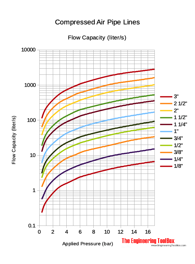
shows a capacity of the compressed air line of \(\sim\SI{2}{\liter\per\second}\).
Thus, we can safely assume the calculated \(\SI{3.25}{\liter\per\second}\) to be a worst case scenario.
Hence, the total amount of air introduced into the system is:
\(n_{\text{total}} = n_{\text{initial}} + \frac{Q_{\text{comp. air}} \cdot \SI{5}{\second} \cdot p_{\text{atm}}}{R T_{\text{amb}}}\), where \(Q_{\text{comp. air}} = \SI{3.246}{\liter\per\second}\)
Ends up to be:
\(n_{\text{total}} = n_{\text{initial}} + n_{\text{flow}} = \SI{0.0069}{\mol} + \SI{0.666}{\mol} = \SI{0.673}{\mol}\)
Given in volume at normal conditions, this results in a gas volume of
\(V_{\text{gas}} = \SI{16.4}{\liter}\)
24.3. Consider pumping of pumps
Since the pumps were still running during this period, they would have extracted most of the gas immediately again. See last point in previous section.
24.4. Calculation of possible contamination
Finally, given the total vacuum volume and the amount of gas, which entered the system, we can estimate the potential contamination.
With the vacuum volume and the gas flowing into the system, the maximum possible contamination can be estimated. The upper limit is of course all contaminations in the gas forming a monolayer in the whole vacuum system. Assuming a certain ppm contamination in the gas, the maximum contamination is simply
\(d_{\text{cont}} = \frac{n_{\text{total}} R T_{\text{amb}} \cdot q_{\text{cont}}}{A_{\text{vacuum}}}\)
where \(q_{\text{cont}}\) is the ppm contaminiation in the total gas volume \(nRT\), which enterd, while \(A_{\text{vacuum}}\) is the total surface area of all vacuum tubing.
However, first we estimate the amount of oil, which entered the system from a typical oil contamination in compressed air. The ISO standard ISO 8573-1:2010 defines different classes for compressed air in different applications. Classes regarding oil contamination range from 0 to 4, with class 4 being the worst. Class 4 calls for \(\text{ppmv}_{\text{oil}} \leq \SI{5}{\milli \gram\per\meter\cubed.}\). Thus, even if CERN's compressed air is a lot worse than this, \(\text{ppmv}_{\text{oil}} \approx \SI{10}{\milli\gram\per\meter\cubed.}\) should be sufficient as a baseline.
This means the entered air will contain about
import math
let air_vol = 16.4
let ppmv = 10e-3
echo ppmv * air_vol
0.164
which is \(\SI{0.164}{\mg}\) of oil.
The telescope surface is not known exactly. No time to find out until this needs to be done. Can be checked again later with Jaime / find slides, paper about LLNL telescope, to get better numbers. Assuming 10 quarter shells of a radius of \(\SI{5}{\centi\meter}\) (some larger, some smaller radius), the telescope has an area of:
import math
let A = 10.0 * 0.5 * PI * 0.05 * 0.5
echo A
0.3926990816987241
, i.e. an area of \(A_{\text{telescope}} = \SI{0.393}{\meter\squared}\). If all of the oil was placed on the telescope, this would result in
import math
let A = 0.393
let oil_mg = 0.164
let ratio = oil_mg / A * 1e-4
echo ratio
4.173027989821883e-05
A contamination of \(d_{\text{max, cont}} = \SI{41.73}{\nano\gram\per\cm\squared}\) is an upper bound on oil on the telescope. Realistically, the telescope only has \(< \frac{1}{10}\) of the total vacuum surface area, while probably \(> \SI{90}{\percent}\) of the oil will have left the system via the pumps, pushing the contamination as low as \(d_{\text{cont}} < \SI{0.4173}{\nano\gram\per\cm\squared}\).
This may still sounds like quite a bit, but the assumptions made here are all extremely conservative:
- 5 seconds with an open valve. More likely it was about \SI{3}{\second} => factor of \(3/5\).
- flow of compressed air of \(\SI{3.25}{\liter\per\second}\), more likely about \(\SI{2}{\liter\per\second}\) => factor of another \(2/3.25\).
- area of telescope vs total area of gas volume (hard to calculate due to flexible tubing) probably quite a bit less than 1 / 10 ?
- \(\SI{10}{\percent}\) of oils sticking to surface probably also extremely unlikely. Maybe 2 orders of magnitude less?
let factors = (3.0 / 5.0) * (2.0 / 3.25) * 0.5 * 1e-2
echo factors
echo factors * 0.4173
| 0.001846153846153846 |
| 0.0007704000000000001 |
Meaning values as low as \(d_{\text{cont}} < \SI{0.7704}{\pico \gram\per\cm\squared}\) may even be more reasonable. It is probably safe to say that this level is easily reached if the telescope sits open during installation etc.